
arXiv Dive: How Flux and Rectified Flow Transformers Work

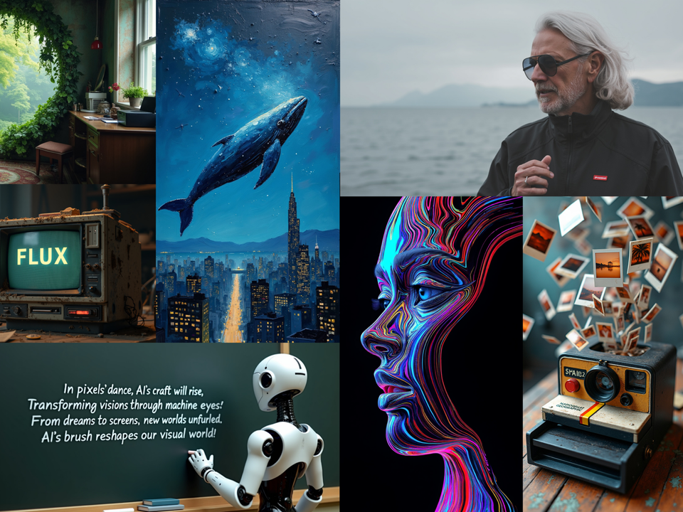
Flux made quite a splash with its release on August 1st, 2024 as the new state of the art generative image model outperforming SDXL, SDXL-Turbo, Pixart, and DALL-E. While the model doesn't have a paper itself, Black Forest Labs, a team made of ex-Stability AI folks, does give a list of their previous papers that influenced their work.
After digging into the open source code, we decided to dive into the Scaling Rectified Flow Transformers for High-Resolution Image Synthesis paper because the architecture is most similar to this paper and it has many of the key concepts.
If you'd like to watch our dive while reading along, here is our recording:
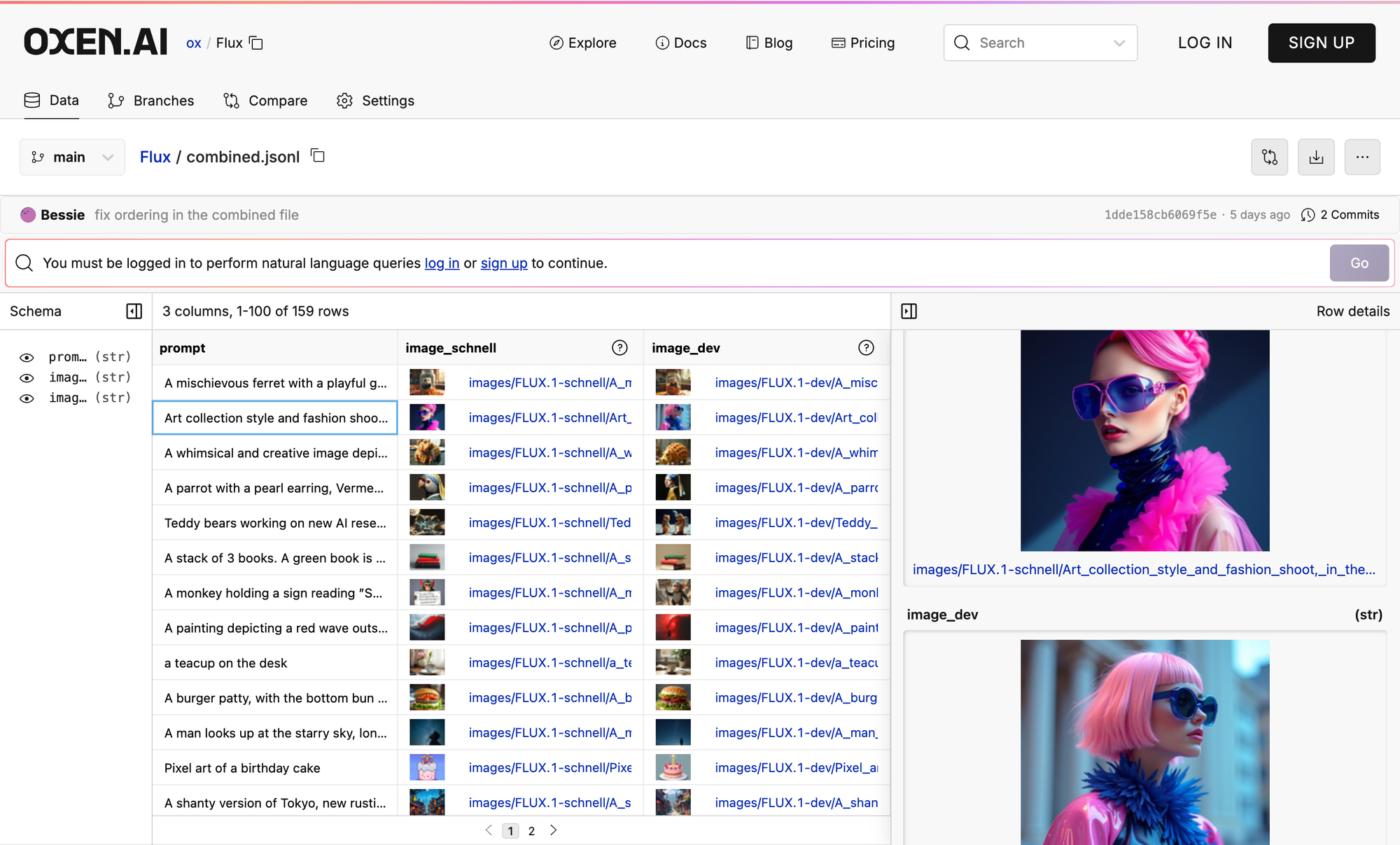
For fun, we took all the prompts mentioned in the paper and ran it through the Flux Schnell (smallest), Dev, and Pro models. Even Schnell got some super impressive results. If you want to compare the different model results or use the data, its absolutely free:)
We are also are midway through tested out AI-Toolkit to fine-tune FLUX with LORA on our Teeny Icon Dataset to try to generate Icons in this style.
While not the most impressive so far, here are some results. We will showing our finished work in our next Water Cooler hour.

Diffusion Models
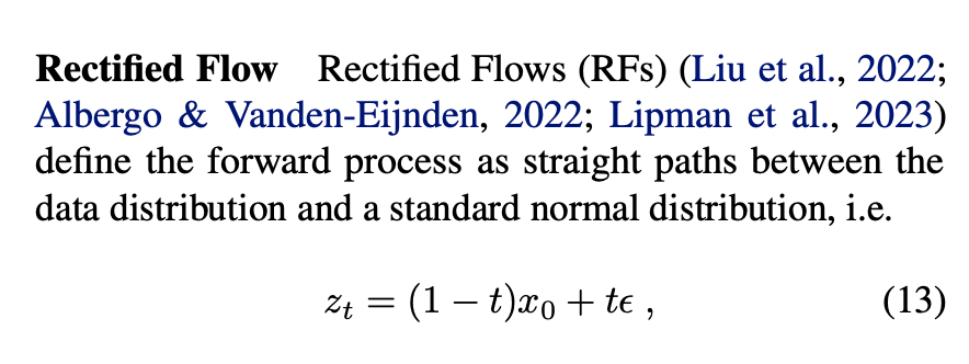
“Rectified flow” is a term we need to build our way up to. They say it is a technique that “connects data to noise in a straight line”.
What does this mean?
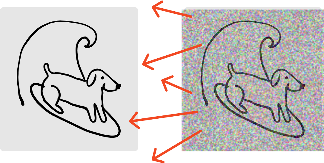
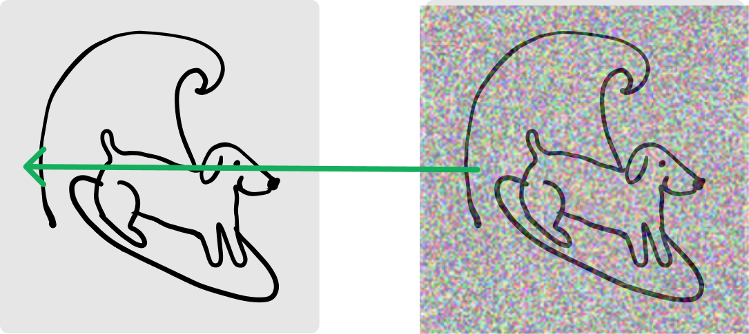
As a refresher - all diffusion models are trained to do is to go from random noise + a prompt to a realistic looking image like so:
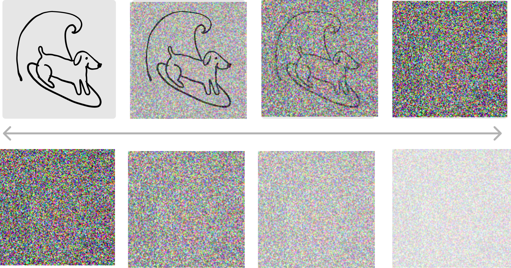
Basically, you have training data that has an image, apply random noise to the image again and again and again, then you have the model subtract the noise and see how well it is able to reproduce the starting image. Seems linear, but curiously it isn't. Let's look at the loss equation of the "rectified flow" paper to understand the difference.
In the loss equation, we find this inner most part:
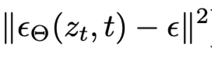
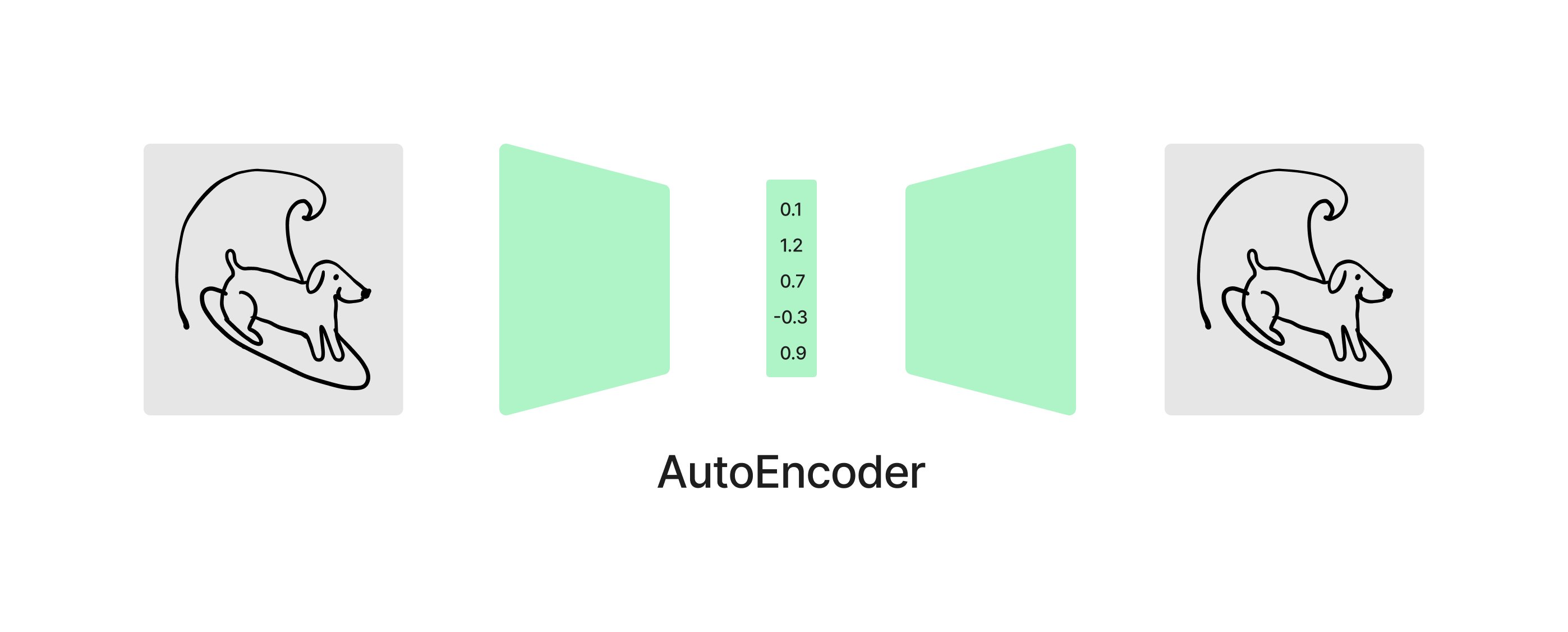
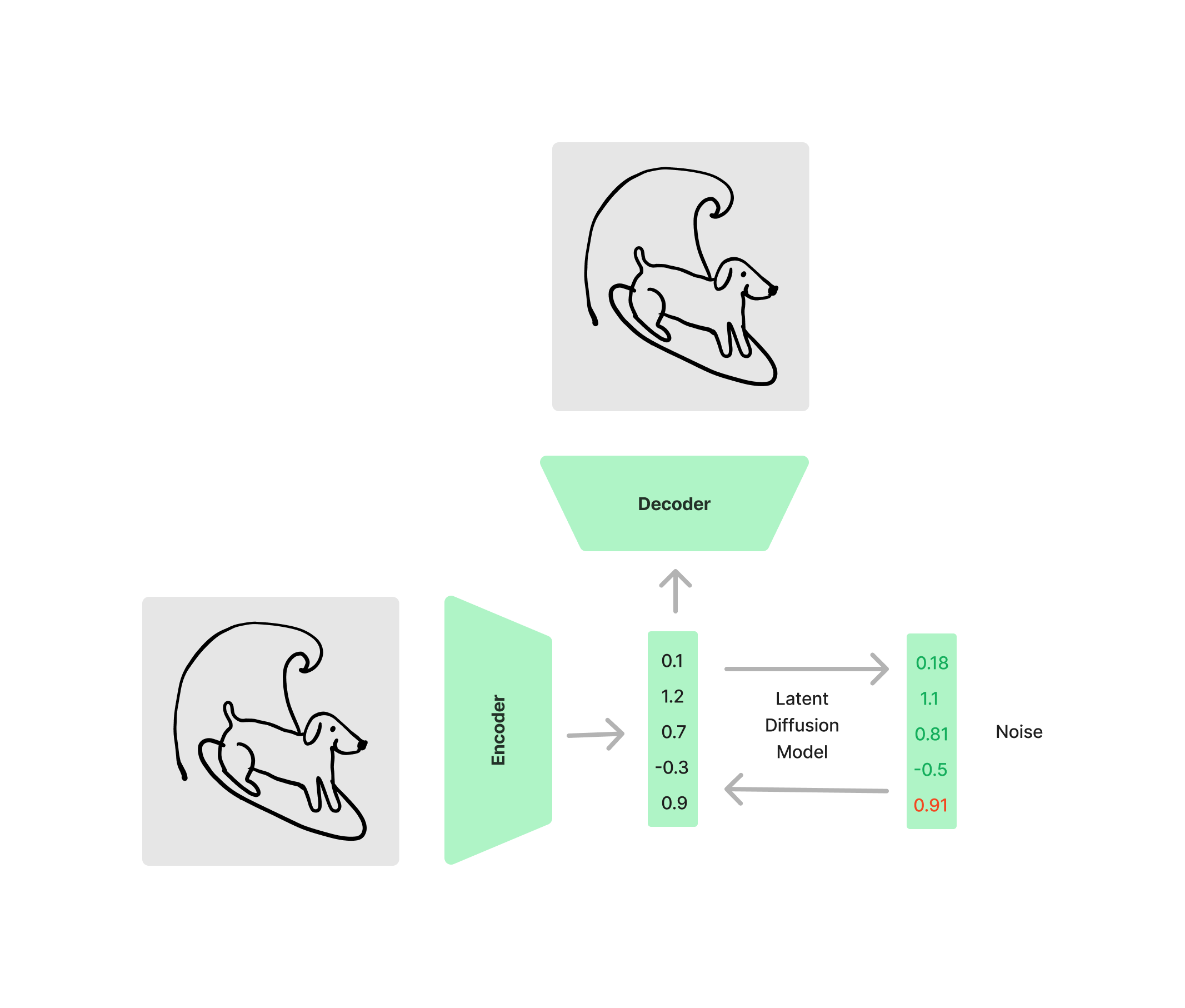
All this is saying is that we subtract some noise (epsilon) from the model’s predicted noise, and take the Mean Squared Error to see how well the model predicted the noise. Now you will notice that the function takes in Z_t, which represents a “latent” variable at time-step “t”. Conceptually it is easy for us to think of diffusion as working in pixel space, but really these are latent diffusion models that actually work in “latent space”. Before you get started you train an auto-encoder to encode the image down to a smaller set of values, that you can then reconstruct the image back from.
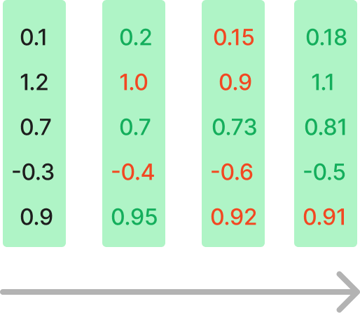
So in latent space the noise might look like this
And then you have to use the decoder half of the auto encoder to go back out from the latent space to the raw image.
If you would like to go deeper into diffusion before "rectified flow", we do have a blog on Stable Diffusion which may interest you.
Importance of Noise Samples and Sample Steps
The paper Common Diffusion Noise Schedules and Sample Steps are Flawed highlights how in flawed diffusion models, the images generated would have very washed colors like in the example below.
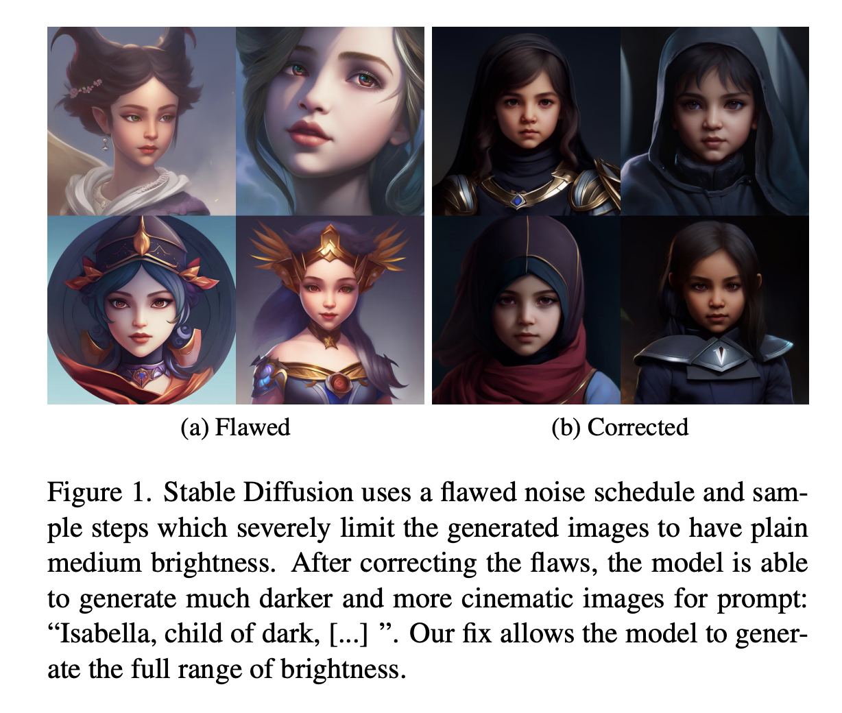
Here Stable Diffusion 1 generated images with medium brightness. The way they sample the noise prevents it from generating very bright and dark samples. This paper argues that specifying a forward path from data to noise leads to efficient training, but it also raises the question of which path to choose. This choice can have important implications for sampling.
“Rectified Flow” tries to connect data and noise on a straight line. But what does this mean?
Flow Trajectories
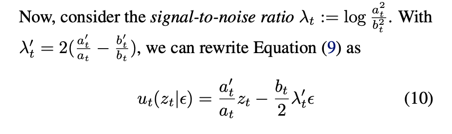
Sections 2&3 of the paper talks a lot about Ordinary Differential Equations (ODEs) and “Flow Trajectories” or velocities. Diffusion papers do a great job of making the math look really intimidating…but let’s try to get an intuition for what is going on here.
You’ll recognize the MSE on the right hand side, the rest looks like gibberish, but we’ll get back to it.
Let’s think about what we are trying to learn at every pixel value. We are trying to learn which way to shift the noise to make the image look more realistic.
The reason we take multiple steps is so that if our original guess isn’t correct, we can course correct along the way. This multiple steps to get to the correct answer is the ODE process, sometimes referred to as Euler’s method to estimate the curve.
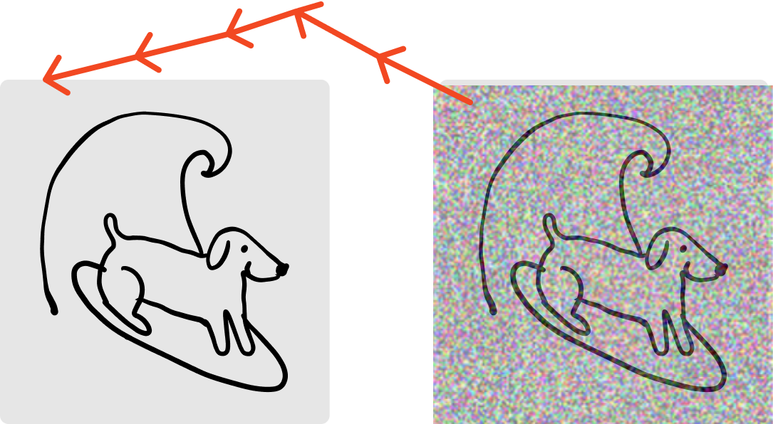
Our ideal state for the trajectory, flow, or velocity, is just a straight line.
You’ll notice in the paper they try many different “flow trajectories” but the one that performs the best is the “Rectified Flow”, which is….a straight line.
So if you think of when t=0, z_t = x0 and when t=1, z_t = t_e (or the noise). All this fancy math is doing is trying to draw that straight line as fast as possible by letting the model learn the “velocity” in which to move next given a time step t. In reality we never really take “one straight line step” to the right answer, if we could, we’d be done. Instead we let the model course correct along the way.
Then, zooming back out to our loss function.
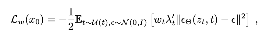
All the first half of the equation is saying is average over all time steps and a unit gaussian distribution for the noise.
t = 0.0, 0.1, 0.2, 0.3, 0.4 …
N = noise
Lambda_t is the signal to noise ratio to let the model know how much signal there should be in the image vs how much noise.
Lambda times W_t is really just a weighting function for which time step you are at.
Intuitively, what they are saying here is that if we are at time step 0 or N (beginning or end of the diffusion process) it is relatively easy to know if you should predict a lot of noise or a little noise. If you are in the middle of the steps it is like half signal and half noise. So this W helps the model “pay more attention” in the middle steps. So when T is in the middle of 0..1 (0.5) W is going to be higher, meaning the loss is going to be higher, and the model needs to do a better job predicting the noise.
Even Pi in this equation above is defined by another equation called logit normal sampling. This is where it gets over my head, but you will see they tried a bunch of lognorm values as hyperparameters later in the paper.
They also compare the “rectified flow” to many other equations for how to go from the image to the predicted noise within that z_t. “EDM”, “Cosine”, “LDM-Linear”, “Tailored SNR”, “CosMap”…but we don’t have time to go into all of them, let’s just ride the winner.
I would just say be thankful they ran all the experiments and compute and tested all these different equations for us so that we don’t have to 😅
Whew, okay, we got auto-encoders, diffusion models, and what this rectified flow thing is trying to do. Now let’s take a look at the whole transformer.
Rectified Flow Transformers
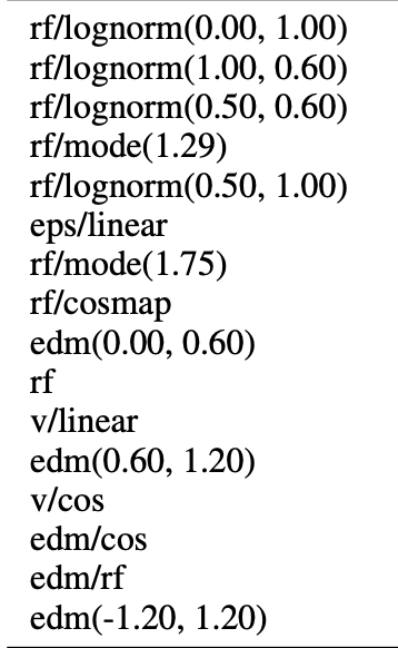
The first thing to notice is the model uses two separate sets of weights for the two modalities, and has two parallel paths that the information from each modality flows down.
There is then attention between all the image and text tokens in the middle of each MM-DiT block. The rest is actually pretty similar to most diffusion transformer architectures like the ones we have covered in previous dives.
Text-To-Image Architecture
Start with a pre-trained auto-encoder and CLIP model so that we can train the text-to-image models in the latent space of the auto encoder. You’ll notice in this model they use multiple CLIP models and a T5 model to encode the text and send it through a linear layer to combine all the features.
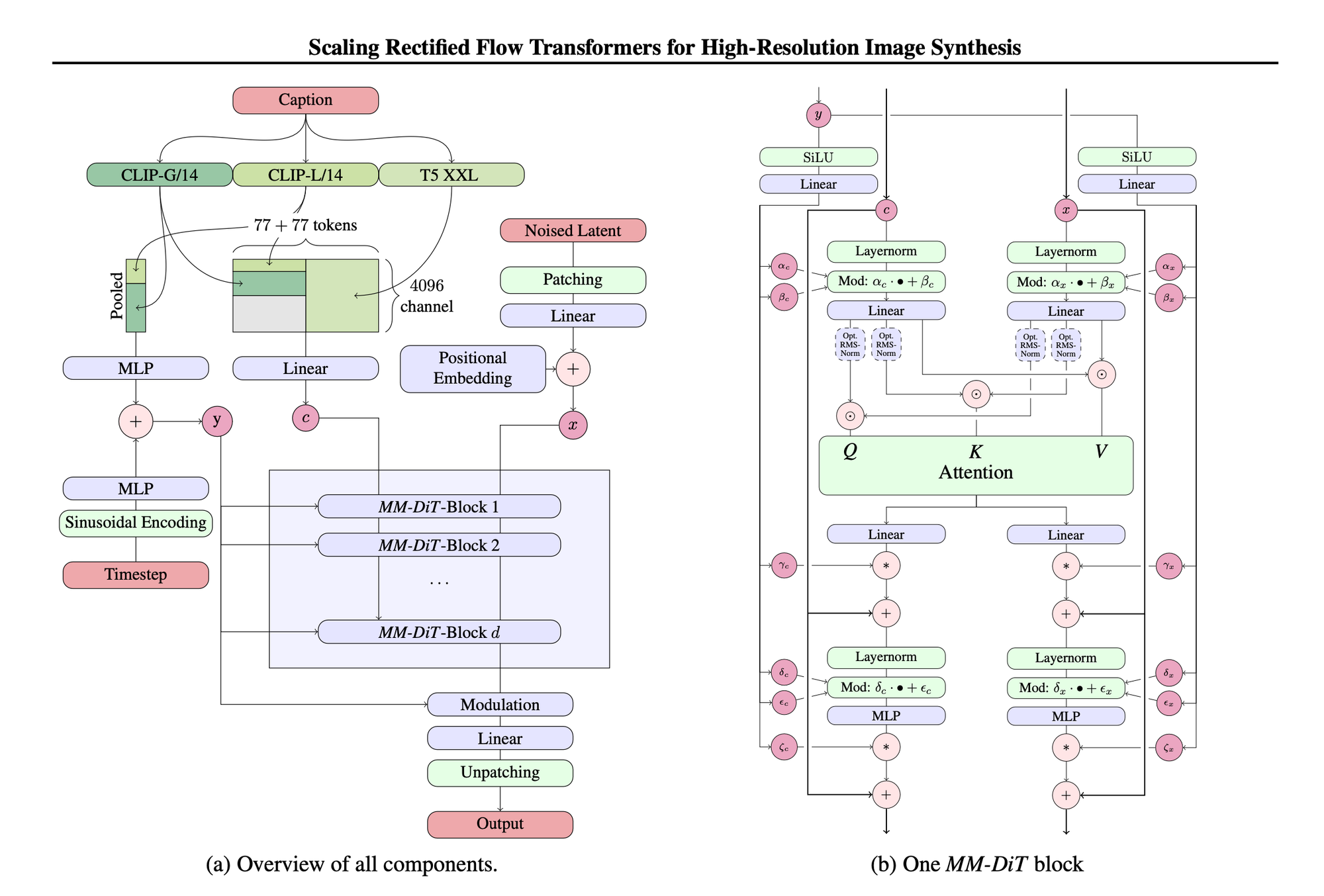
They call the transformer blocks MM-DiT blocks that stand for Multi-Modal Diffusion Transformer blocks. Someone on Reddit looked at the code for Flux and drew out a flow chart of it’s model, and it looks pretty similar to the one above.
Datasets
The used ImageNet - “a photo of a {class name}” (1.4m images with labels) and CC12M dataset (Conceptual 12M: Pushing Web-Scale Image-Text Pre-Training To Recognize Long-Tail Visual Concepts).
Auto Encoder Size
The auto-encoder is an important part of any generative image model and is usually pre-trained before the diffusion training begins. The latent space goes from HxWx3 in pixel space to hxwxd in latent space where
h = H/8
w = W/8
d = 16
So for a 512x512x3=786,432 image it is translated to a 64x64x16=65,536 latent space which 12x smaller space.
2562563=196,608
323216=16,384
Which is also a factor of 12
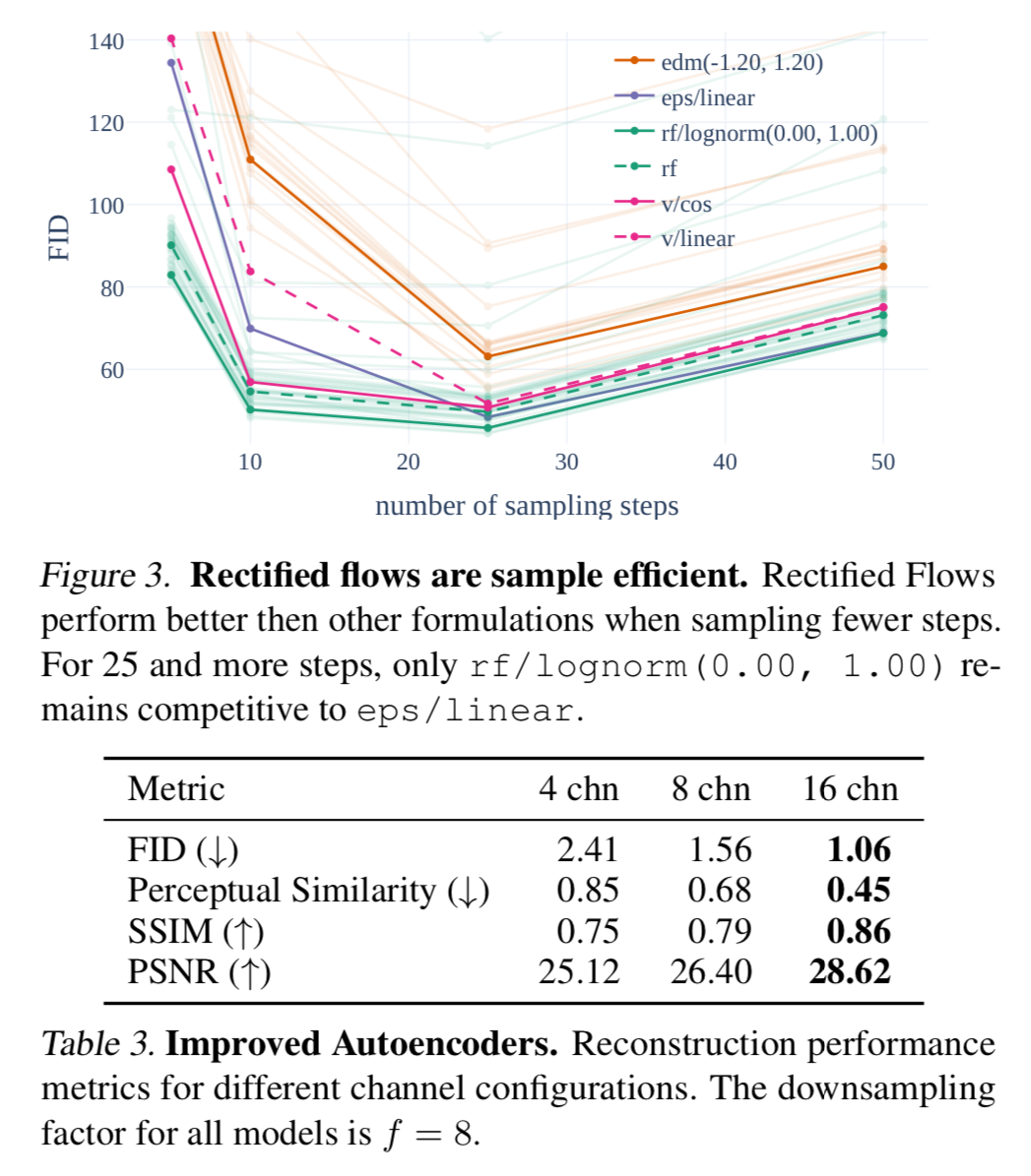
They say that “intuitively, predicting latents with a higher d is a more difficult task, thus models with increased capacity should be able to perform better for larger d, resulting in higher image quality”
They use a d=16 (see figure 10)
At depth=22 the gap between 16ch and 8ch becomes negligible.
Improved Captions
Betker et al (2023) showed that synthetic captions can greatly improve generative image models at scale.
This is often due to the simplicity of human captions. Remember - the original training data for generative image models were alt tags on html pages. Humans are lazy when tagging images, and omit details describing the foreground, background, composition of the scene etc.
They take an off the shelf, state of the art vision-language model CogVLM to create synthetic annotations and create a 50/50 % training split of original and synthetic captions.
Data Preprocessing
They filter out NSFW, images with low quality (based on model predictions) and deduplicate similar data using semantic clustering and deduplication.
Since the model uses the output of multiple pretrained, frozen networks (auto-encoder and text-encoder) they precompute all of the embeddings before training to save on compute during training.
Positional Encodings
They use 2D frequency based embeddings for the positional encodings so they use a combination of extended and interpolated position grids which are the frequency embedded. What does that look like?
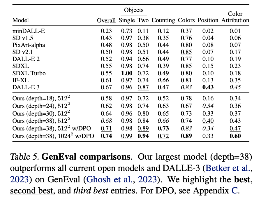
Results
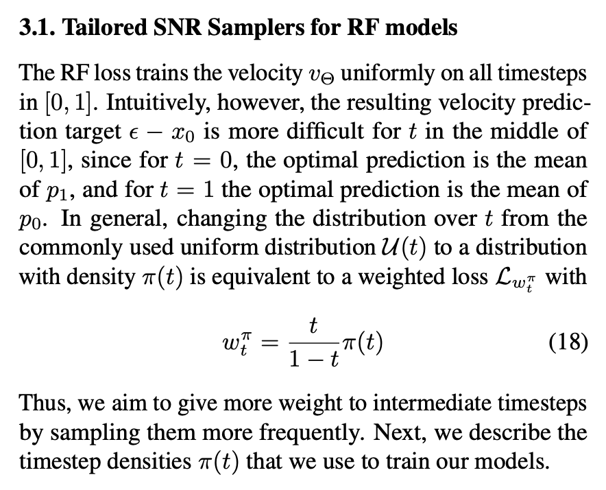
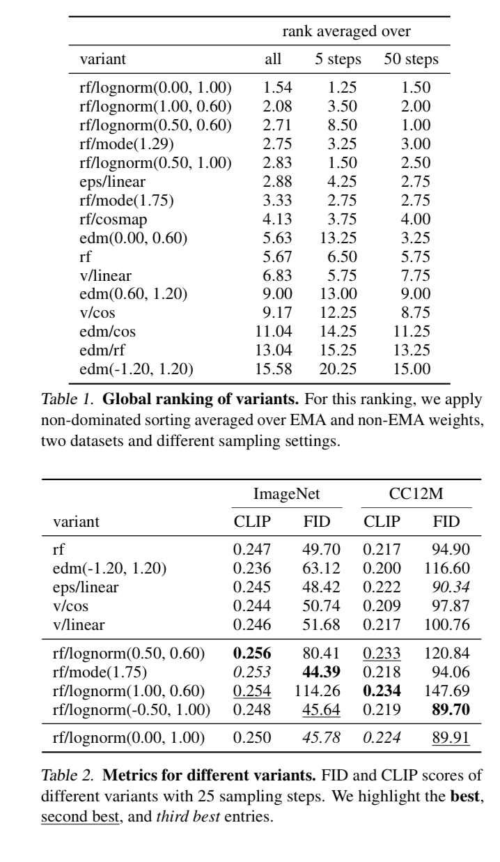
Rectified flow with lognorm(0,1) seems to perform the best consistently.
They also report their scores on GenEval which is a cool evaluation framework
https://arxiv.org/abs/2310.11513
Conclusion
So the TLDR, they used synthetic data for improved captioning, they have a multimodal diffusion transformer block that takes in the text and images and has separate pipelines that communicate with each other through attention, and they have the rectified flow equation to guide the model to be straight when choosing its trajectories. Really cool that the model is open source and we can play around and study it.
If you want to see the results of each model, make sure to clone our Flux repo, quickly clone it, and have fun comparing the models!

Member discussion