
How a $1 Qwen3-VL Fine-Tune Beat Gemini 3

Can a $1 fine-tune beat a state-of-the-art closed-source model?
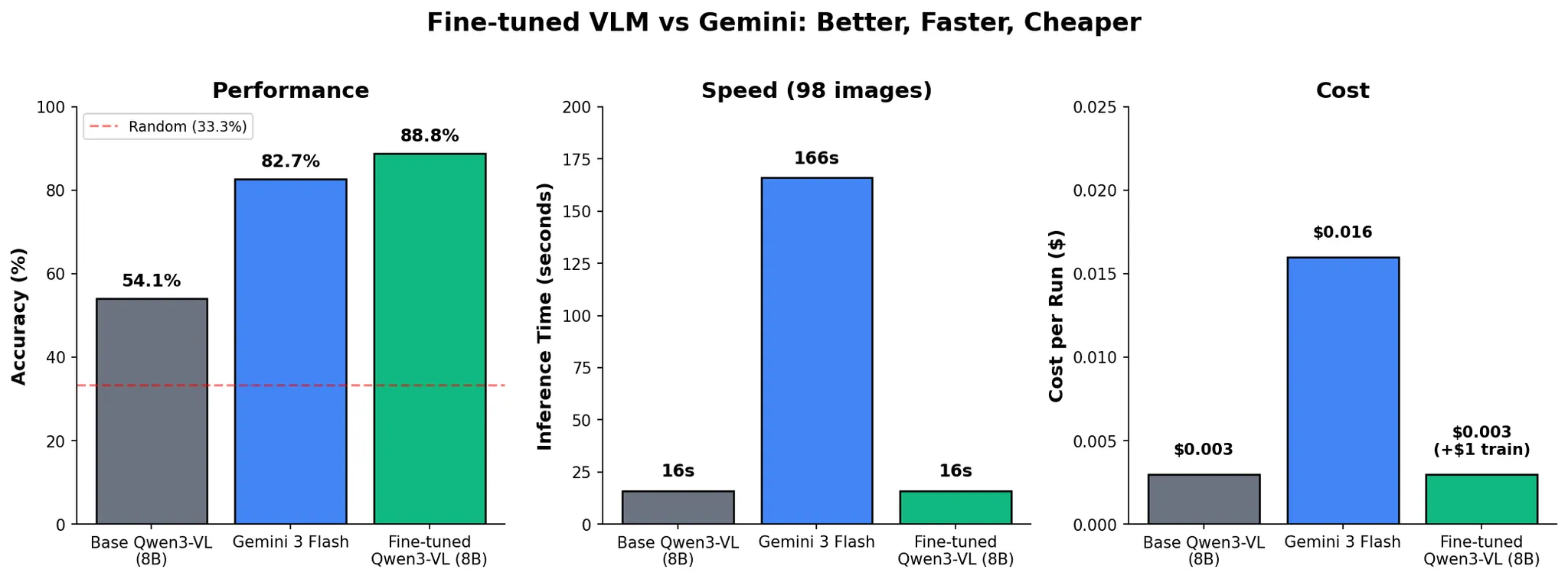
| Model | Accuracy | Time (98 samples) | Cost/Run |
|---|---|---|---|
| Base Qwen3-VL-8B | 54.1% | ~10 sec | $0.003 |
| Gemini 3 Flash | 82.7% | 2 min 46 sec | $0.016 |
| FT Qwen3-VL | 88.8% | ~10 sec | $0.003 |
Spoiler: yes, let us show you how!
If you find this content interesting, feel free to join our live Fine-Tuning Friday sessions, where we walk through real world AI use-cases live. Here's a recording from last session, which unfortunately we forgot to smash the record button on, but Eloy kindly took the time to film again!
Why VLMs?
Before we dive in: quick little recap. What are Vision-Language Models?
VLMs combine vision with language understanding. They take images + text as input and produce text as output. Great for captioning, labeling, describing, and many other tasks. The applications are everywhere:
- Insurance: Classify car damage, validate claims, flag fraud
- Healthcare: Identify abnormalities in X-rays, MRIs, pathology slides
- Manufacturing: Spot defects on production lines in real time
- Media & Entertainment: Scan video frames for unwanted brands or logos
- Retail: Automated quality inspection and inventory counting
- Agriculture: Detect crop disease from drone imagery
The Setup
It's no surprise that we at Oxen.ai are big fans of open-source models, and we have a lot of fun fine-tuning them. Continuing our tradition (which began when we showed how efficiently Qwen-Image-Edit can be fine-tuned), we wanted to put Alibaba's Qwen3-VL to the test and see how it stacks up against a heavyweight closed-source model from one of the other top labs.
Car damage detection is a real problem, and not just for folks like me browsing Facebook Marketplace. Insurance companies process thousands of damage claims daily, and manually reviewing photos is slow and expensive. A model that can automatically classify damage types could save these companies hours of work (and tons of money). Let's see if we can build one.
The task is simple:
Input: Photo of damaged car
Output: One of three classes: scratch, dent, crack
This is a pretty interesting challenge for a few reasons. Labeling this type of damage is tough even for humans, the visual differences between a crack and a scratch are subtle, and a dent with scraped paint can easily be mistaken for either.
The sheer scale of the problem makes it very cost-sensitive. Insurance companies process thousands of claims daily, and even saving a few cents per inference request can translate to millions of dollars in savings. On top of that, new accidents happen every day, so the data you're processing will constantly drift outside the training distribution. The model needs to actually learn the task, it can't get away with memorizing samples.
And of course prompt engineering gets tough when you're passing in images as input. The context gets saturated fast and performance tends to be terrible. This is actually a great indicator that fine-tuning is worth exploring, if you can't prompt your way out of a problem, fine-tuning is usually the next lever to pull.
The Dataset
Luckily, I don't have to scrape together a damage dataset from Facebook Marketplace myself. I can use CarDD (Car Damage Detection), a publicly available dataset out of USTC containing ~4,000 high-resolution images with multiple annotation types, originally designed for detection and segmentation.
One small problem: remember how this is supposed to be a quick test? Let's downsample this dataset a bit.
This dataset includes many images with multiple damage types per photo, which would complicate our evaluation. To keep things simple, we filtered down to images with only a single damage category and picked three classes to focus on. Worth noting: we absolutely could train Qwen3-VL on multiple labels, Oxen.ai supports multi-category labeling out of the box, but for this proof of concept, single labels keep things clean.
| Original CarDD | Our Subset |
|---|---|
| ~4,000 images | 417 images |
| Detection + segmentation | Classification only |
| Multiple damage types | 3 classes: crack, dent, scratch |
| Complex labels | Single labels |
Here's what our final split looks like:
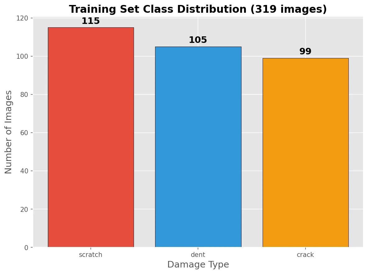
Small, clean, and ready to train. If you want to explore the data yourself, here's the Oxen.ai repo we created to store it.
Time to answer the question:
Can we teach a small open-source model to do this better than a giant proprietary one? (and how?)
A great way to approach this kind of experiment is to follow the recipe laid out by Karpathy in his blog post A Recipe for Training Neural Networks. If you haven't read it, no worries, we'll go over it step by step during this little exercise.
Become One with the Data
"Spend quality time with your data. Look at examples. Understand the distribution. Your brain is surprisingly good at recognizing patterns."
First step in the recipe: become one with the data. Spend more time than you'd be comfortable with just looking at samples, trying to recognize patterns between the images, what can the model realistically learn? How can you improve your dataset to squeeze even better performance out of your fine-tuned model?
One big advantage of using Oxen.ai is that we get to actually see our data, browse it, query it, spot issues visually. And sure enough, we spotted a few problems almost immediately!
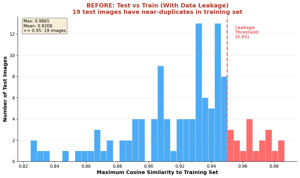
Problem 1: Train/Test Leakage
Remember the cardinal rule? Your eval data should never have been seen during training. Turns out we had near-duplicates sneaking across the split:
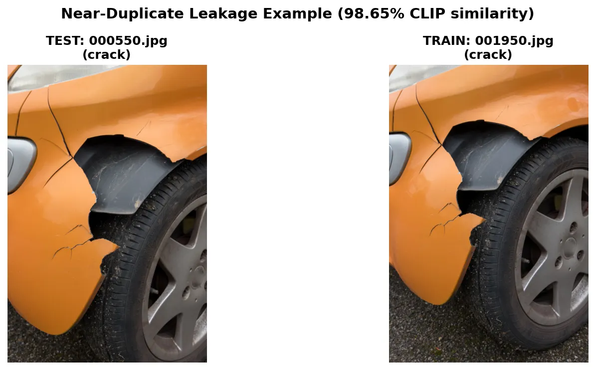
These are essentially the same photo, just slightly different crops. On a massive dataset this might be noise, but on a 417-image sample, that's the kind of leakage that lets a model memorize instead of learn (no bueno).
Trusting our eyes to recognize data leakage is great, but we're smart oxen, why do the work ourselves when we can write a Python script to catch it systematically?
The idea is simple: if two images are nearly identical, their embeddings should be nearly identical too. We used CLIP to embed every image in the dataset and computed cosine similarity between all test-train pairs, basically a score from 0 to 1 that tells you how similar two images are.
Anything above 0.95 is a red flag. We found 126 suspicious pairs, removed 19 leaked test images, and ended up with a clean split of 98 test samples ready for evaluation.
The 0.95 threshold is a bit arbitrary, these similarity scores will naturally run high since we're comparing images of cars with other images of cars. One way to get more meaningful similarity scores would be to fine-tune CLIP itself to produce better-separated embeddings for this domain.
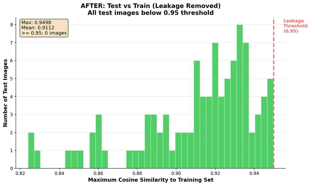
After shuffling and cleaning, no pairs exceeded our threshold. Clean dataset in hand, we can move on!
Problem 2: Multi-label Reality
Here's the other thing we noticed: the subset of the dataset we chose uses single labels, but real car damage is often multi-class. A crash that dents the metal usually also scratches the paint. We used majority-vote labeling from the original annotations, but keep this in mind when we get to the "impossible" images later.
What Does the Data Look Like?
Here are some examples from each class:
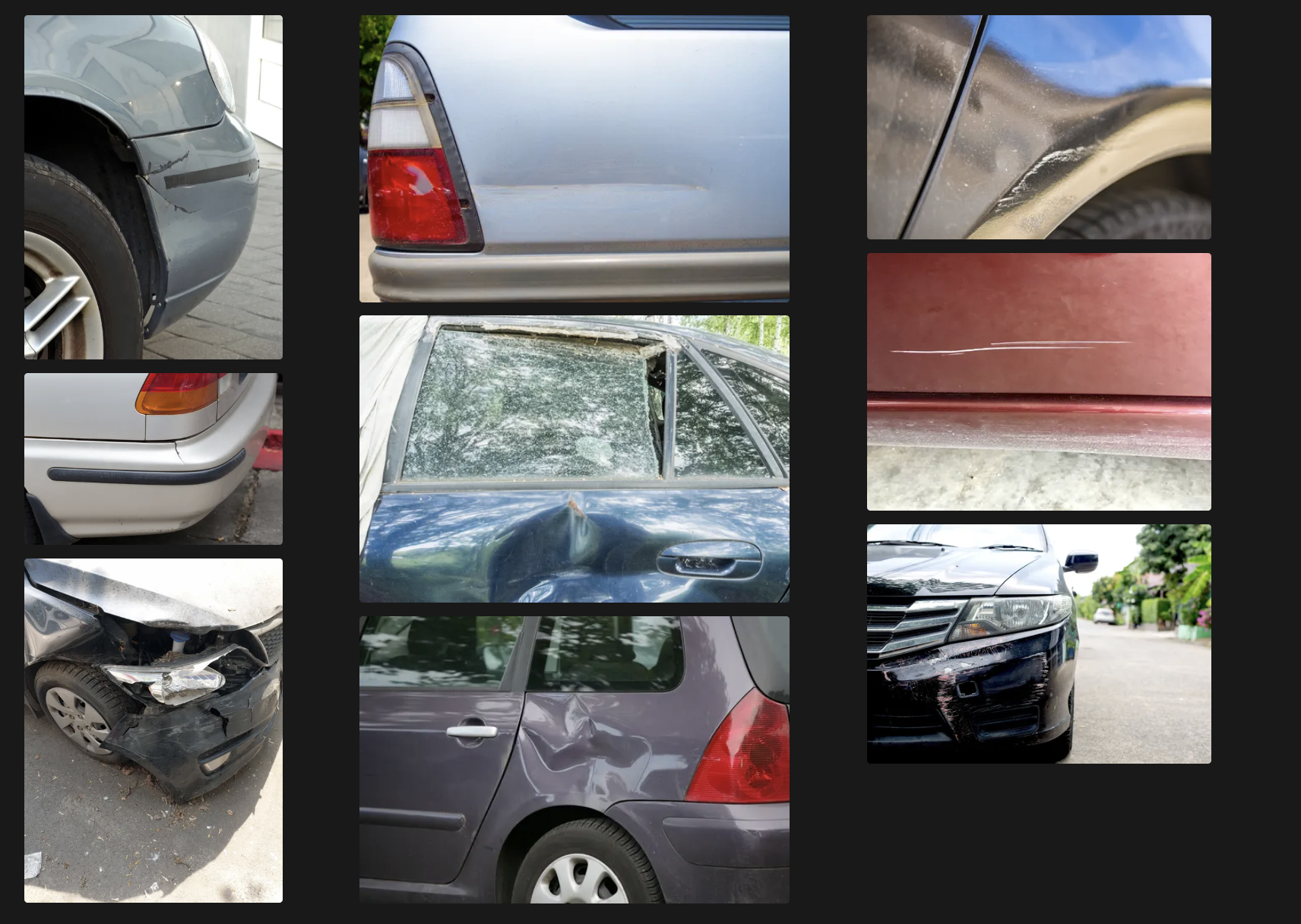
Key observation: cracks are the hardest to distinguish. A little intuition we can get from just looking at the data is that when a car visibly has several damage types, cracks tend to take precedence in the labeling, this is a quirk of the dataset itself and might be why cracks are so hard to predict.
How VLMs Actually Work
Before we start training, let's quickly understand what we're fine-tuning. A Vision-Language Model has three main components:
Image → [Vision Encoder] → [Projection Layer] → [LLM Backbone] → Text
1. Vision Encoder (ViT): Chops the image into patches (think a 14x14 grid), then produces an embedding vector for each patch. These are your "image tokens."
2. Projection Layer (MLP): The vision encoder and the LLM speak different "languages", their embedding spaces have different dimensions. The projection layer is just an MLP that maps vision vectors into the same dimensional space as text tokens. It's not learning semantics, just translating coordinate systems.
3. LLM Backbone (Qwen): Here's the key insight, image tokens and text tokens get concatenated into a single flat sequence, and standard self-attention runs over the whole thing:
[img_patch_1] [img_patch_2] ... [img_patch_N] [text_tok_1] [text_tok_2] ... [text_tok_M]
The model doesn't care which tokens came from an image and which came from text. Every token attends to every other token. When the model processes "What damage is this?", the text tokens can attend to image patches showing the crack, and vice versa. No special cross-attention mechanism, the model learns to relate modalities purely through regular self-attention.
Setting Up Training + Baselines
"Get a simple training loop running. Establish baselines before doing anything fancy."
We need a number to hillclimb against, baselines are very important when it comes to evals.
VRAM Back-of-the-Napkin Math
This is a good rule of thumb we use at Oxen.ai to decide what's the best GPU to run a particular model on. When you use Oxen, you don't have to think about this, we pick the GPU that gives you the best cost efficiency, so you know you're not leaving money on the table.
Nevertheless, it's a good concept to keep in mind, as you can estimate a ballpark of how much inference will cost.
| Precision | Bytes/Param | 8B Model | 70B Model |
|---|---|---|---|
| FP16/BF16 | 2 | 16 GB | 140 GB |
| INT8 | 1 | 8 GB | 70 GB |
| INT4 | 0.5 | 4 GB | 35 GB |
Qwen3-VL-8B at BF16 = 16 GB base. Full fine-tuning needs ~3x for optimizer states = 48 GB.
Baselines
Here's how different models performed out of the box:
| Model | Accuracy | Notes |
|---|---|---|
| Random guess | 33.3% | 3 classes |
| Base Qwen3-VL-8B | 54.1% | Zero-shot |
| Gemini 2.0 Flash | 78.6% | API call |
| Gemini 3 Flash | 82.7% | API call |
The base model is barely better than random on cracks, only 19.4% correct! Let's look at the confusion matrix:

The model straight up doesn't know what car cracks look like. It keeps calling them scratches or dents.
Overfit First (The Sanity Check)
"Verify your model can learn. Overfit a tiny dataset to loss ~0."
Before training on the full dataset, we need to prove the model can learn. This is a quick sanity check to make sure the training pipeline has no bugs and the data is in the correct format and properly flowing through.
- Take 10 training samples
- Train for 100+ steps
- Watch loss go to ~0
View the overfitting run on Oxen.ai
If this fails, it's a bug in your code or data, not the model. Ours went to ~0 as expected. We're good to go.
VLM Quirks We Discovered
These are a few quirks we discovered while overfitting the model during our initial implementation.
Quirk 1: Loss stalls and won't go down
We had completion_only_loss=False, which meant the model was penalized for not predicting image tokens. But it's not an image generator! Once we set it to only compute loss on the text output (also known as train_on_input=False or mask_prompt=True on other frameworks), training started working properly.
Quirk 2: Training looks good, inference = base model
We trained LoRA on Qwen3-VL, loss decreased beautifully, everything looked great. Deployed with SGLang, applied LoRA at runtime... and results were nearly identical to the base model.
The culprit? SGLang's LoRA filter only matches LLM layers, not vision layers:
# From sglang/srt/models/qwen3_vl.py
_lora_pattern = re.compile(
    r"^model\.layers\.(\d+)\.(self_attn|mlp)\.(qkv_proj|o_proj|...)$"
)
Only model.layers.{N}.* matches, vision modules like visual.* get silently skipped! We had to merge the LoRA weights into the base model instead of applying them at runtime.
Using Oxen.ai means you don't have to spend hours debugging cryptic performance issues like this. We feel the pain so you don't have to.
Tune
"Now train on the full dataset, adjust hyperparameters, and iterate."
Here's where the fun begins!
LoRA:
We add these small matrices to attention layers throughout the model. The original weights stay frozen, and the adapter outputs get summed in.
LoRA Hyperparameters Deep Dive
These are the main hyperparameters you might want to play with when fine-tuning a LoRA for Qwen3-VL. You can change all of these when training on Oxen.ai, though we give you smart defaults so you can get going without thinking too much about it.
| Parameter | Value | What It Does |
|---|---|---|
| LoRA rank (r) | 64 | Size of low-rank matrices |
| LoRA alpha | 16 | Scaling factor |
| Learning rate | 2e-4 | Step size for updates |
| Batch size | 4 | Images per update |
| Epochs | 3 | Passes through data |
| Target modules | q,k,v,o_proj | Which attention layers to adapt |
We'd recommend experimenting with different values to squeeze out a bit more performance from your tuned model. Once you have a good baseline run you want to improve on, you can trigger as many concurrent experiments as you want by playing around with these values directly on Oxen!
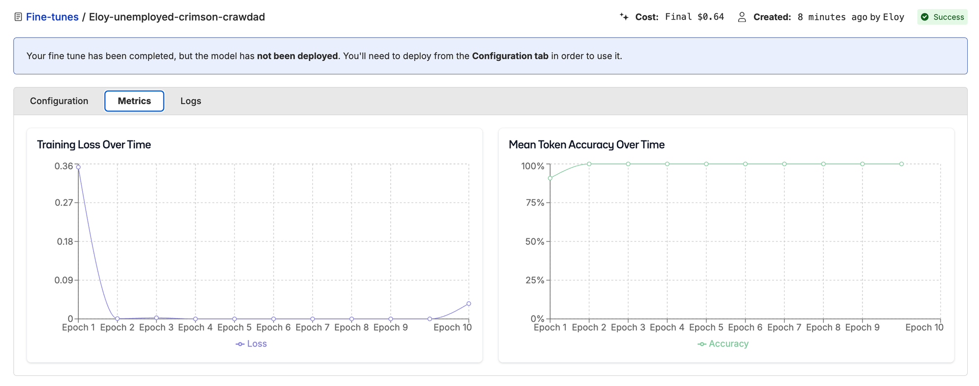
Scaling Up
All we have to do to run these fine-tunes on Oxen is upload your dataset (1–2 clicks), start a new fine-tune, choose which columns of your dataset you want to train on (4–5 clicks), and just wait for the magic! The full 319 sample training run took about 8 minutes and cost just $1!
Here we start to see some interesting results. With these two data points we can start plotting an accuracy curve.
| Training Samples | Accuracy | Improvement | Training Cost |
|---|---|---|---|
| 0 (base) | 54.1% | — | — |
| 78 | 67.3% | +13.2 pp | $0.50 |
| 319 | 88.8% | +21.5 pp more | $1.00 |
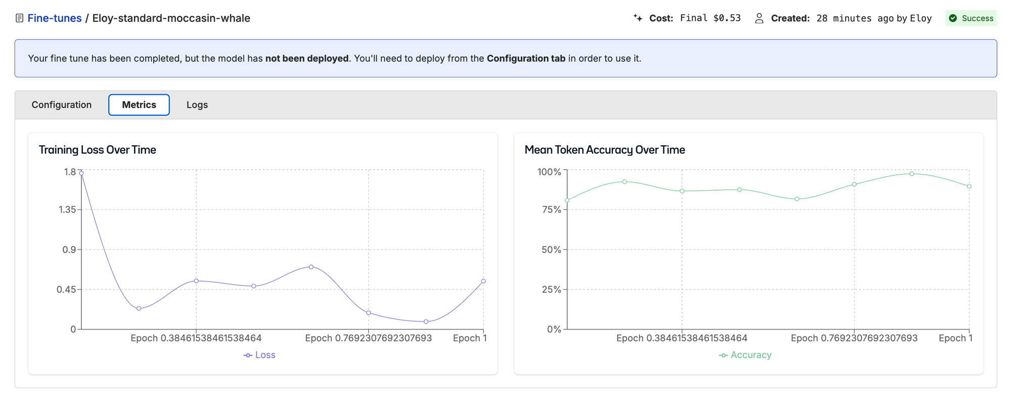
Training loss for 78-sample run.
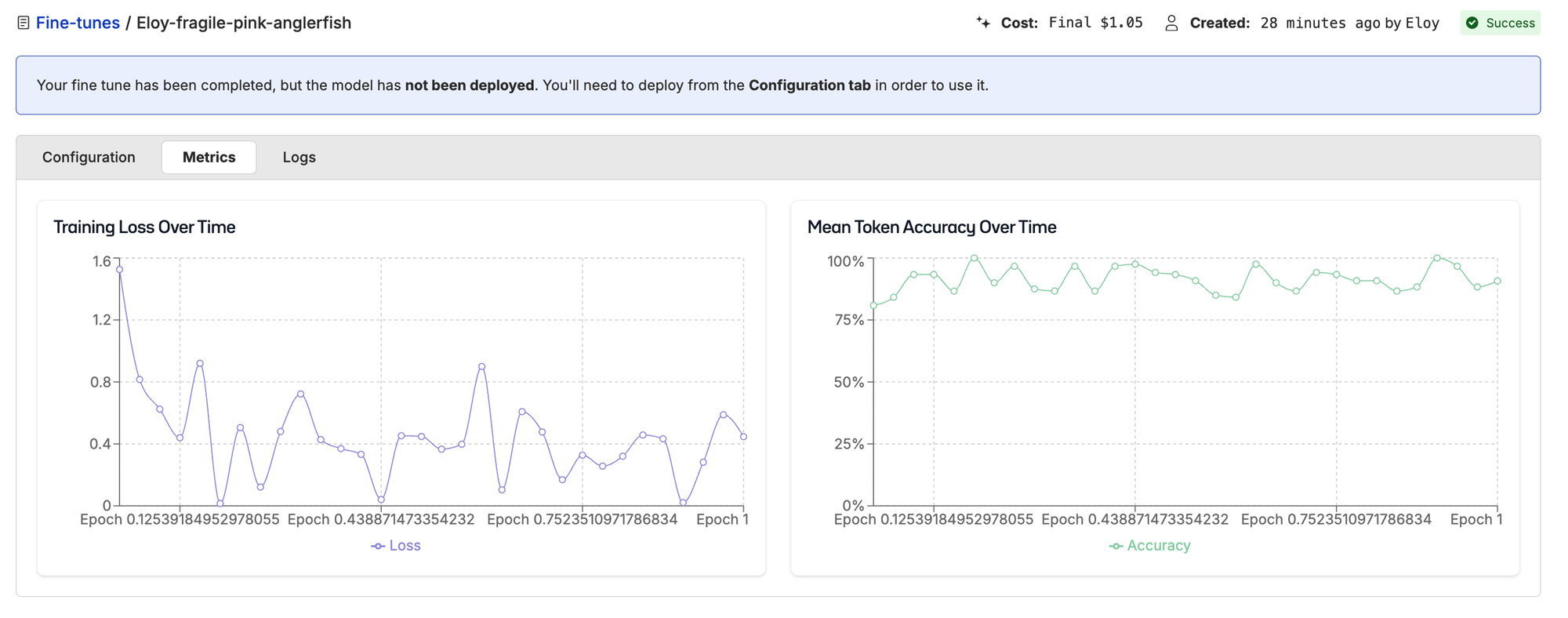
Training loss for 319-sample run.
Turns out the more (clean) data we have, the better results we get, unsurprisingly. But look at where the improvement happened:
| Class | Base | Fine-tuned | Change |
|---|---|---|---|
| Crack | 19.4% | 96.8% | +77.4 pp |
| Dent | 75.0% | 78.1% | +3.1 pp |
| Scratch | 65.7% | 91.4% | +25.7 pp |
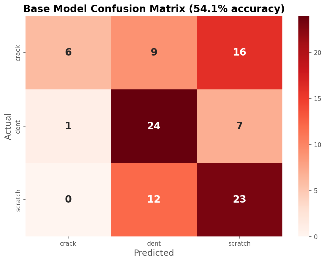
Weak diagonal, the base model struggles.
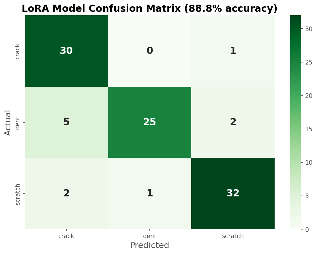
Strong diagonal, the fine-tuned model nails it.
The model went from 19.4% to 96.8% on cracks, a +77 percentage point swing. From the intuition we got from looking at the data, we can safely say the model is now classifying cars with several types of damage as cracks. This might not be the most intuitive thing to do as a human, but once again this is a dataset quirk and might very well be how car insurers are taught to assign single-label damage to claims.
Squeeze Out the Juice
Learning curves typically follow a power law, each doubling of data gives roughly similar improvement. Knowing this, we can use every statistician's favorite party trick, a simple extrapolation, to estimate what our accuracy would look like if we added more data.
This is obviously not deterministic, the accuracy improvement will strongly depend on the quality and type of data you feed into the model and how hard the task is. But from our two data points we can see that accuracy is not yet plateauing, so a surefire way to improve performance would be to add more clean data.
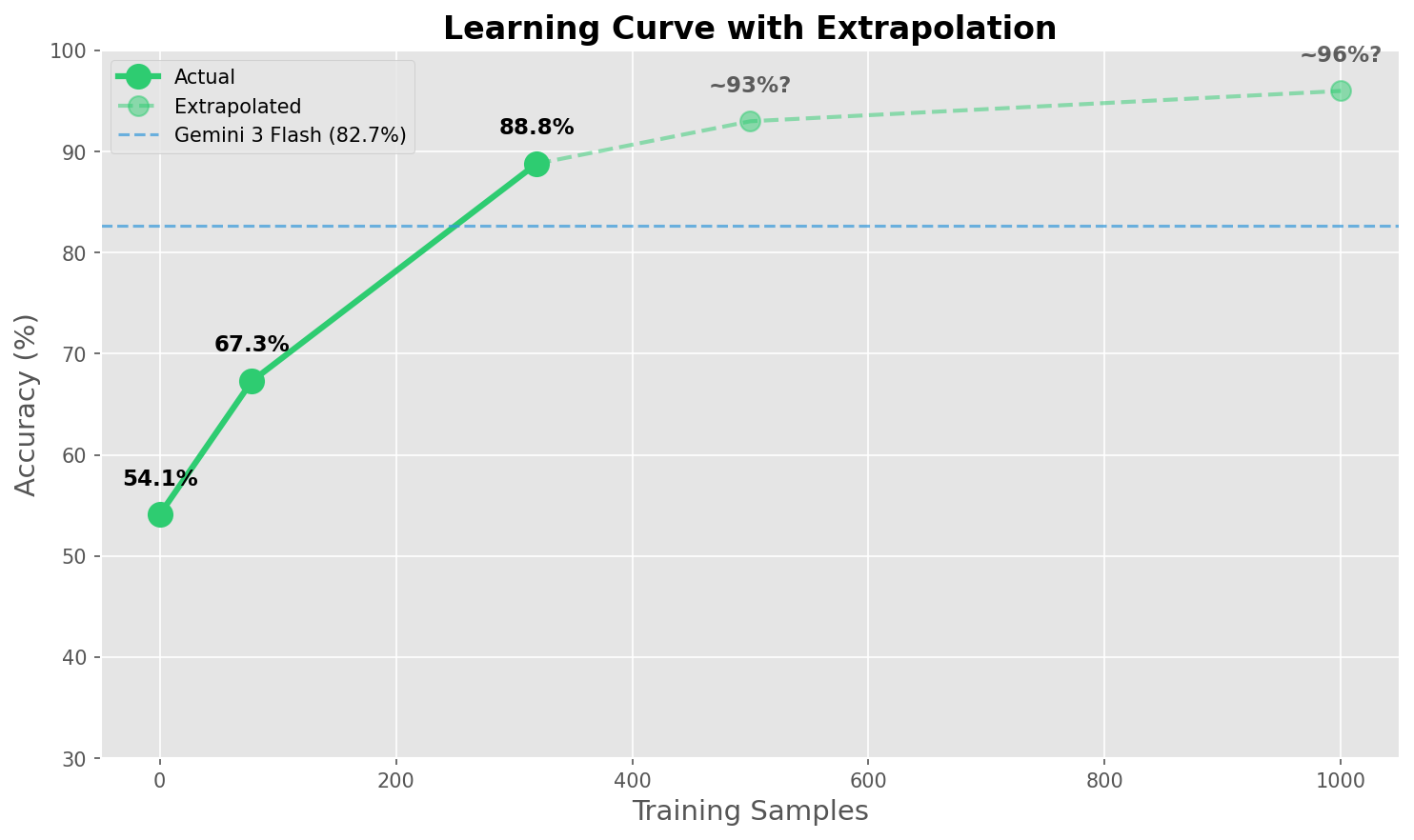
We can clearly see the diminishing returns, the closer you get to 100% accuracy the harder it becomes, and the more data you have to add. At some point you need to evaluate the tradeoff of curating and labeling more data (which is very non-negligible) for ever-smaller accuracy improvements.
What we didn't try (yet):
- More training data (500–1000 samples)
- Larger model (Qwen3-VL-32B)
- Hyperparameter sweeps
- Quantization to lower inference cost
The Results
Let's start with what fine-tuning actually fixed. We tagged every test image in our dataset so you can query them on Oxen.ai:
| Tag | Count | Description |
|---|---|---|
both_right | 48 | Both models correct |
base_wrong_lora_right | 39 | Fine-tuning fixed these |
both_wrong | 6 | "Impossible" images |
lora_wrong_base_right | 5 | Regressions |
Before/After: What Fine-Tuning Fixed
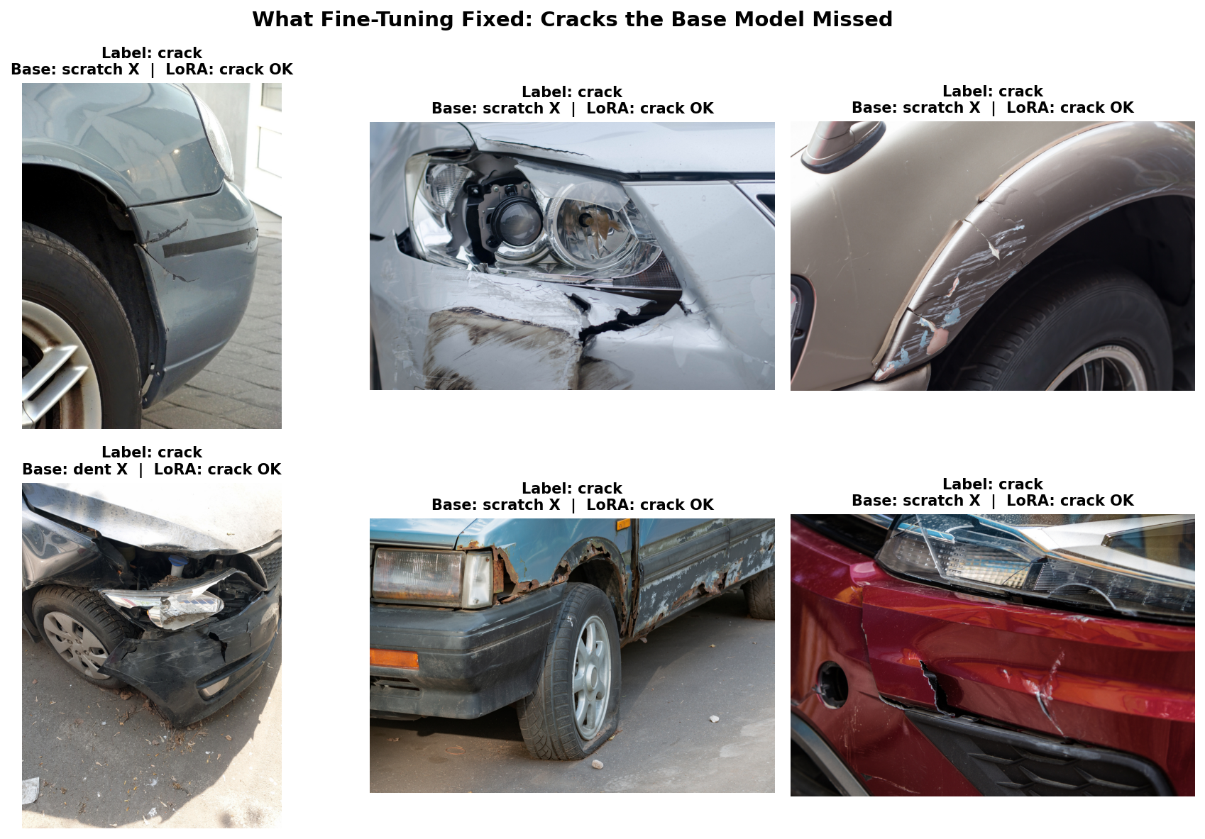
These are cracks the base model couldn't recognize. As we can see, there are a few samples in there that we as humans would have a hard time classifying as just "cracks", but the model learned what the training dataset had to teach, so we'll count that as a win!
Final Scoreboard
| Model | Accuracy | Inference Time | Cost/Run | Training Cost |
|---|---|---|---|---|
| Base Qwen3-VL-8B | 54.1% | 10s | $0.003 | — |
| Gemini 2.0 Flash (batch) | 78.6% | 203s | $0.0015 | — |
| Gemini 3 Flash | 82.7% | 166s | $0.016 | — |
| LoRA Qwen3-VL | 88.8% | 10s | $0.003 | $1 |
We ran Gemini 2.0 Flash through the batch API expecting it to be quicker, turns out that endpoint is optimized for cost, not speed. They give you a 24-hour window to run your inference at a very cheap price. Good for the wallet, terrible for patience.
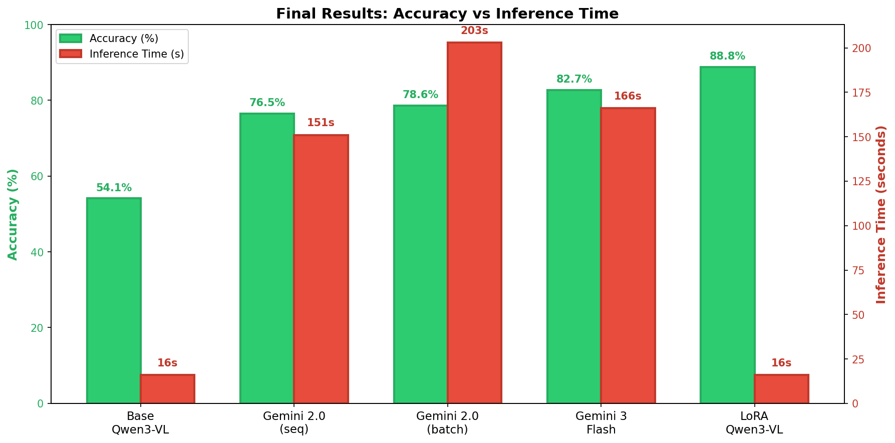
Our fine-tuned open-source model didn't just match Gemini 3, it beat it by 6.1 percentage points. And it did so 10x faster, running on a single A10G GPU. The cost difference might look small here, but it becomes a lot more obvious as you scale up the amount of inference you need to run.
Head-to-Head vs Gemini 3 Flash
| Outcome | Count |
|---|---|
| LoRA wins (we're right, Gemini wrong) | 10 |
| Gemini wins (Gemini right, we're wrong) | 4 |
| Both correct | 77 |
| Both wrong | 7 |
Net advantage: +6 images over Gemini 3 Flash.
The "Impossible" Images
Both models fail on 7 images. Some of these are genuinely ambiguous, even as humans we'd have a hard time assigning a single label to them.
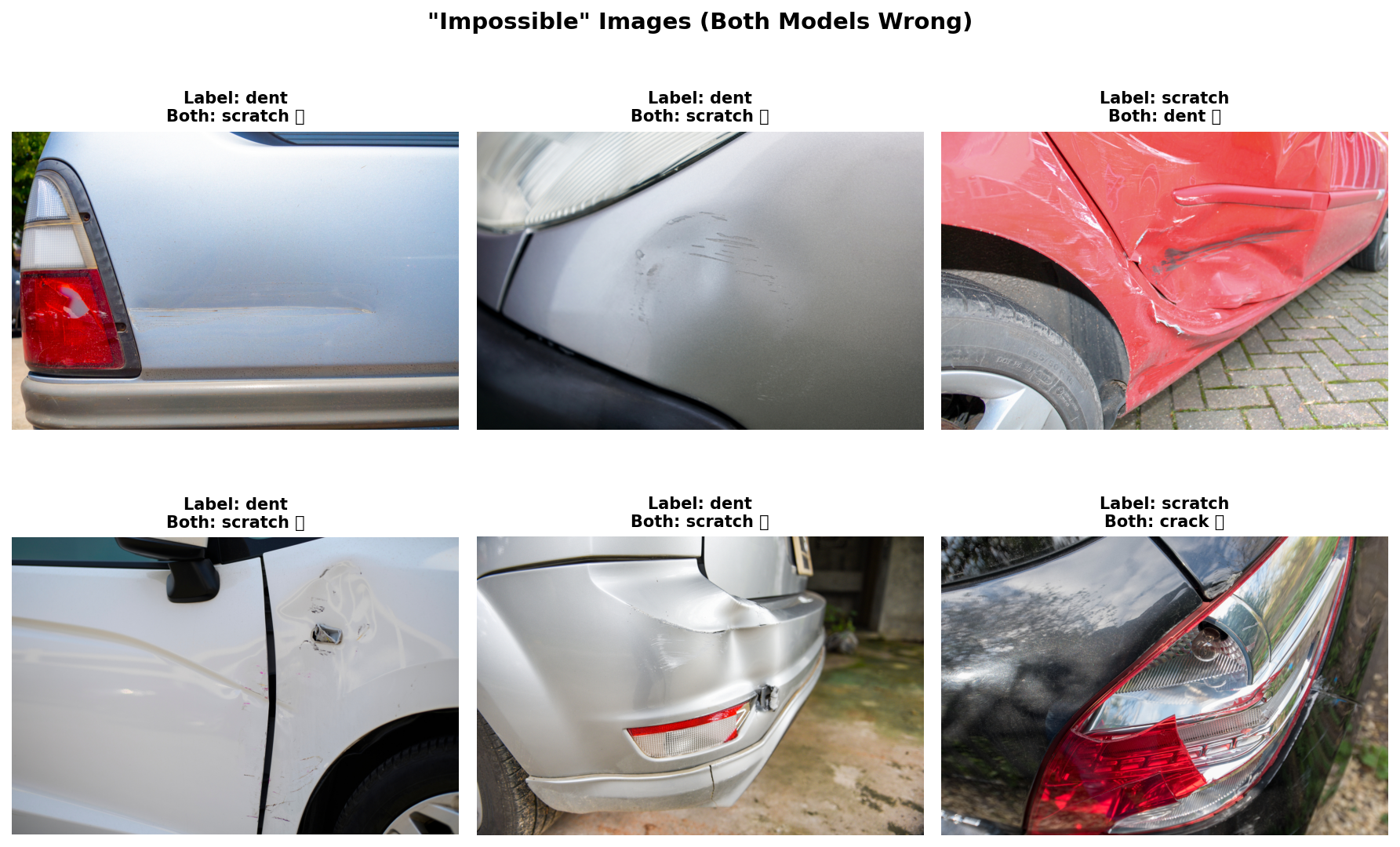
This is exactly why looking at your data matters. When both a fine-tuned specialist and Gemini 3 agree on a prediction that contradicts the label, maybe the label is wrong. By tagging and querying these edge cases on Oxen, you can identify where your dataset needs work: relabel ambiguous samples, add more examples of tricky cases, or rethink whether your labeling scheme reflects the real-world task.
The Honest Caveats
Let's be real about limitations:
| Caveat | Context |
|---|---|
| 98 test samples | Small, but balanced across classes |
| 87 vs 81 correct | Only 6 sample difference |
| Single domain | Car damage only, not general vision |
But the direction is clear:
- 88.8% vs 82.7% = consistent gap
- More training data → more improvement (not plateauing)
- 10x faster inference is real
What this proves: Domain-specific fine-tuning on small open models can compete with general-purpose giants.
What this doesn't prove: That this works for every domain or that you don't need more data for production.
The Takeaway
Following Karpathy's recipe works:
- Become one with the data - Found leakage, understood class imbalance
- Set up baselines - Base model: 54.1%, Gemini: 82.7%
- Overfit - Verified the pipeline works
- Regularize - LoRA gives you regularization for free
- Tune - More data helped (88.8% with 319 samples)
- Squeeze - Batch inference, merged weights
| Benefit | Value |
|---|---|
| Accuracy | +6 pp over Gemini 3 Flash |
| Speed | 10x faster (10s vs 166s) |
| Cost | Time is money |
| Privacy | Data stays on-prem |
| Control | Full model ownership |
The Pragmatic Path Forward
Here's what we've learned: it makes total sense to start with a big lab model. When you're prototyping, Gemini or GPT-4V gives you zero setup, instant results, and a high baseline. Don't pre-optimize, validate the idea first.
But eventually you hit walls. Cost at scale ($0.01/image x 1M images/month = $10K/month), latency (API calls adding hundreds of milliseconds), privacy concerns (sensitive data leaving your infrastructure), and an accuracy ceiling you can't break through with prompt engineering alone.
That's when fine-tuning becomes worth the investment. And the best part? It doesn't have to be painful.
Using Oxen.ai means you don't have to wrangle dependencies, fight CUDA driver issues, or debug cryptic inference bugs. Upload your data, click fine-tune, deploy. What took us days of debugging takes minutes on the platform.
A $1 fine-tune on 319 images beat Google's best model by following a simple recipe. And that's now accessible to everyone.
So what are you waiting for? Come fine-tune Qwen3-VL, or any other model, on Oxen.ai. Fine-tuning is powerful, accessible, and (as we just showed) surprisingly cheap. We'll keep proving it in upcoming posts. Stay tuned!
Member discussion