
Arxiv Dives - How LoRA fine-tuning works
Every Friday at Oxen.ai we host a paper club called "Arxiv Dives" to make us smarter Oxen 🐂 🧠. We believe diving into the details of research papers is the best way to build fundamental knowledge and keep up with the bleeding edge. If you would like to join the discussion live, sign up here.
The following are the notes from the live session. Feel free to follow along with the video for the full context.
Background Knowledge
Paper: https://arxiv.org/abs/2106.09685
Published: October 16th, 2021, by Microsoft and CMU
This one is going to be the most math heavy one yet, and requires some basic linear algebra. Luckily the linear algebra is adding and multiplying numbers, which I am confident we all know how to do.
I’m going to start by high level going over the math and why, then we can dive into the details of the paper, and how they apply it to transformers such as GPT-2 and GPT-3.
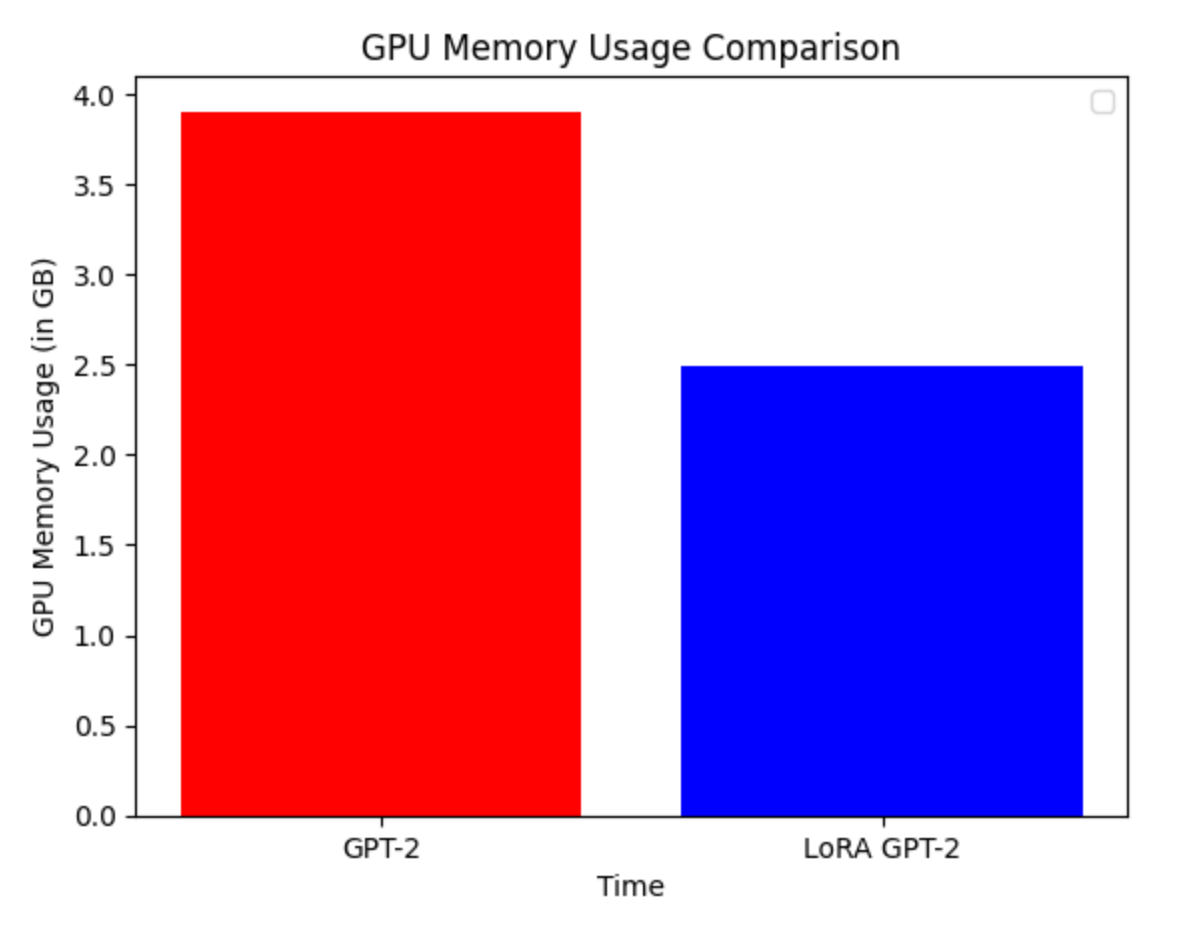
The main takeaway: LoRA reduces the number of trainable parameters, which results in a decrease in training time and GPU memory usage, while maintaining the quality of the outputs.
LLMs are (by their name) extremely large in size. Fine-tuning datasets are often much smaller than their pre-training datasets. LoRA relies on updating a much smaller set of weights, which is advantageous when you have a smaller dataset.
How LoRA Works
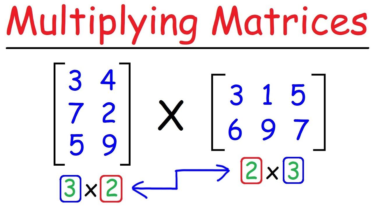
If you are familiar with matrix multiplication, an AxM * MxB matrix, turns into a AxB matrix.
Assume we have an MxM pre-trained dense layer (weight matrix) W, somewhere in a neural network.
For example, this Keras Model has 3 dense layers of size 512x512 each:

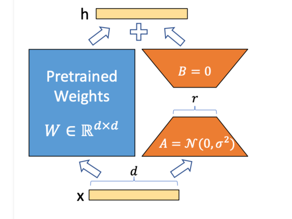
We initialize two more dense layers, A and B, of shapes M x R, and R x M, respectively.
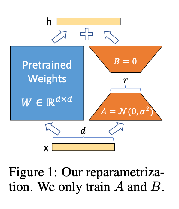
R (rank) is much smaller than M. In the paper, values between 1 and 4 are shown to work well.
So if we take some actual numbers, maybe your dense layer is 512x512= 262,144 parameters.
You could have a 512x4 and a 4x512 which are each only 2048 parameters each, for a total of 4096 parameters.
The original equation of a dense layer is:
Y = Wx + b
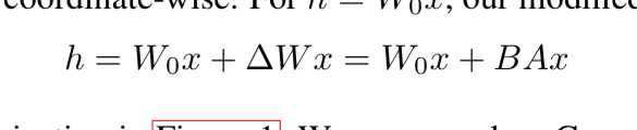
LoRA modifies it to be:
Y = Wx + b + BAx
Where x is a 512x1 vector that is the input to your network and b is a 512x1 bias vector.
Seeing the the matrix multiplication math lines up:
  Dimensions of each variable:
  W = 512x512
  x = 512x1
  b = 1x512
  B = 512x4 (New params)
  A = 4x512 (New params)

  Dimensions fully laid out:
  Y = (512x512) * (512x1) + (1x512) + (512x4) * (4x512) * (512x1)
But in this case we are only training A and B matrices, which are 2048 parameters each. So our number of trainable parameters reduces from 262,144 to 4,096 weights.
What parts of a neural network can we optimize?
When training/running a neural network, there are a few places we need to consider how much memory we are using.
- Total model size
- Size on disk, size over network for serverless, size in RAM, size on GPU, size on CPU
- Inference batch size
- Batch size, sequence length, data size.
- Memory needed for training
- All the model parameters + the gradients for the trainable parameters.
If you recall how backpropagation works, you need to also compute every partial derivative and store them in memory for the backwards pass. This means you are doubling the memory usage for a traditional full fine tuning.
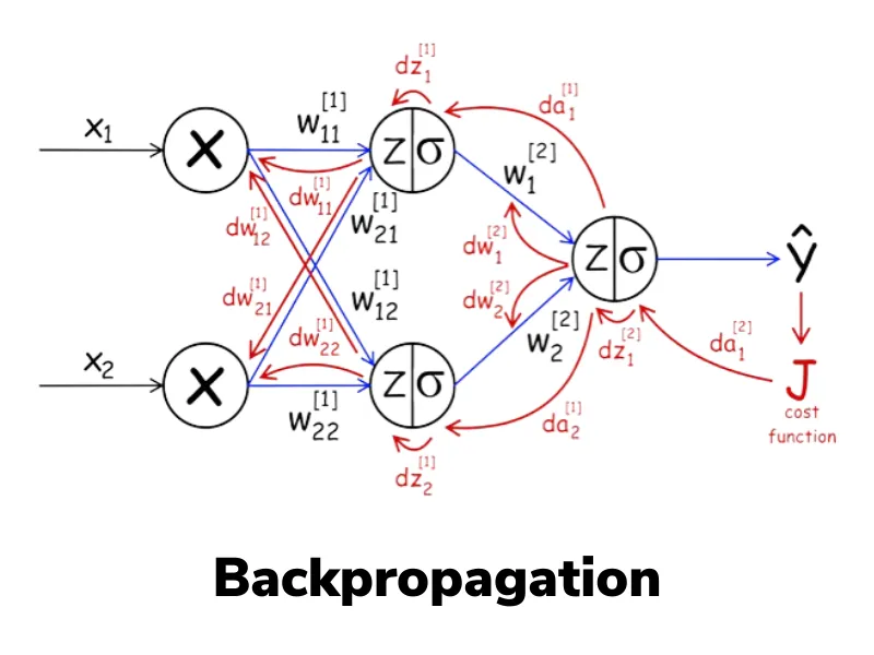
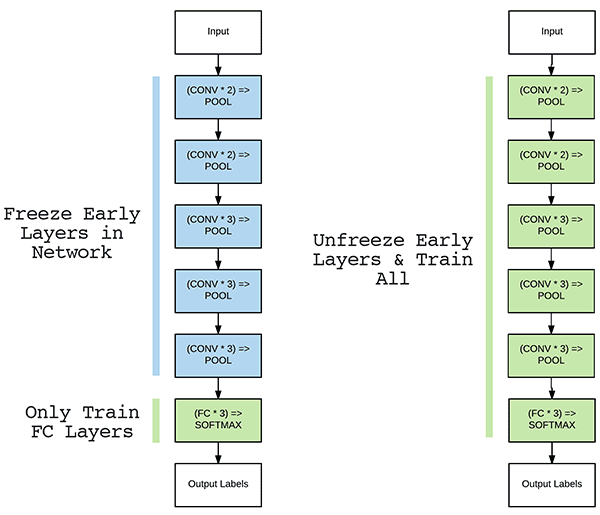
LoRA reduces the total memory needed for training, by only training the rank decomposition matrices (A and B).
These small set of adapter weights, that can be merged into the actual model itself, so it doesn’t affect inference or total model size at all.
Why is there no additional inference time?
The original LoRA equation is:
Y = Wx + b + BAx
We can rewrite this because of the transitive property of addition.
Y = Wx + BAx + b
Or factor out the x as:
Y = (W + BA)x + b
Which means we can simply add (W + BA) to get our new W1 and get back to the original linear equation.
W1 = (W + BA)
We are back to the original equation, with a new set of weights.
Y = W1*x + b
This means that if we merge the weights of the original model and the adapter, we will be essentially doing the same computation as the original model!
Diving Into The Paper
The current paradigm of natural language processing is pre-training on a large corpus of general data, then fine-tuning to a specific task or tasks. With large models, full fine-tuning of all the parameters becomes prohibitively expensive.
If you use GPT-3 as an example, which has 175B parameters, this means you now need to double that to store all of the gradients for training, let alone if you want to store multiple fine-tuned models you need to save each one off with it’s full set of parameters.
LoRA can reduce the number of trainable parameters 10,000x and the GPU memory requirements by 3x.
In practice, it really depends on your model size how much the memory usage decrease is.
LoRA performs on-par or better than fine-tuning despite having higher training throughput and no additional inference latency.
Introduction
Many applications in NLP rely on adapting one large-scale general model to multiple downstream applications.
For example, you might have a general model that can complete a lot of English sentences with the most common next words. The problem with the human language is there are many valid continuations for the same sentence.
Think about how many different opinions people have on different topics. A lot of it is based on their past experiences, and we constantly battle it out in the space of ideas.
The same thing goes for language models. Say you want a downstream model that can summarize text in your voice, or be able to translate natural language to SQL queries, or make a fine-tuned model funnier than the base model, you can do this via fine tuning.
One of the downsides of fine-tuning an entire model end to end, is that the new model contains as many parameters as the old model. If you want N fine-tunes, that means linearly increasing the storage and memory for each new model.
Some have solved this problem by learning external modules for new tasks, or adding new layers to the end of a neural network, but this adds inference latency.
What is "Rank" in LoRA?
They lean into the fact that over-parameterized models reside in a low intrinsic dimension and hypothesize that change in weights during model adaptation has a “low intrinsic rank”.
The “rank” of a matrix is the number of linearly independent columns or rows within it.
You can think of linear independence in a neural network as “how much new information does each set of weights add to the decision making”.
Rank zero would be a matrix of all zeros.
If you had a matrix that looked like this:
1 2 3 4
2 4 6 8
5 3 9 7
You can see the first two rows are just multiples of each other, so they will continue to point you in the same direction. But the third row takes us in a completely different direction.
In the image below, rank 2 would be a 2 dimensional surface because all the vectors are aimed in the same direction, but rank 3 would be more of a cube because each vector is pointed in a different direction.
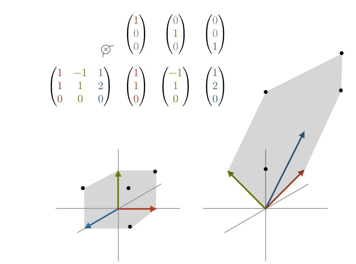
Neural networks have much higher dimensions than 2 or 3, but our brains have a hard time visualizing.
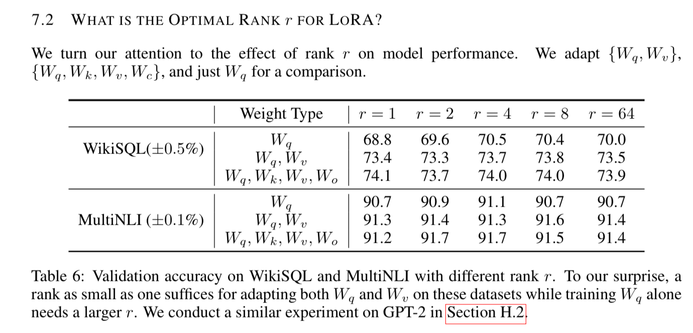
They state that a low rank (even 1 or 2) suffices even when the full rank is as high as 12,228.
The advantages of a technique like this are:
- One pre-trained model can be shared and you can build many smaller LoRA models for different tasks.
- LoRA makes training more efficient and lowers the hardware barrier to entry.
- The simple linear design allows the weights to be mergable, which introduces no inference latency.
- LoRA can be applied to many model architectures and prior methods, since it is a simple dense layer.
In this case, they apply LoRA to the Transformer architecture. So the following section is helpful to know which variables mean what.
Aren’t Existing Solutions Good Enough?
They acknowledge that the problem is by no means new. Transfer learning has many variations on the idea of making model adaptation more parameter and compute efficient.
Specifically they call out “adapter layers” and optimizing input layers or prompts.
Adapter layers even though can be small in size, have to be processes sequentially, instead of in parallel, so do add additional latency.
Low-Rank-Parametrized Update Matrices
They use a random Gaussian initialization for A and zero for B so that B*A at the beginning of training is zero.
They state that LoRA generalizes to a full fine tuning because once you set the LoRA rank to the rank of the pre-trained weight matrices, it converges to training the original model.
When deployed into production you can explicitly compute and store W = W + BA and perform inference as usual. When you need to switch out a fine-tune to another downstream task, you can recover the original W by simply subtracting BA and then adding back in a different one, which is very little memory overhead.
Applying LoRA to Transformers
They only apply LoRA to the weight matrices in the Query, Key, and Value weight matrices of the attention mechanism, and do not apply it to the other dense layers.
They leave applying LoRA to other parts of the transformer as “future work”.
Practical Benefits
The most significant benefits are from reduction in memory and storage.
For GPT-3 175B they reduce the VRAM consumption from 1.2TB to 350GB. 🤯 that training GPT-3 requires that much VRAM.
With r=4 and only the Q and V matrices being adapted, the fine-tune checkpoint sizes are roughly 35MB instead of 350GB…so 10,000x reduction.
Note you still need the 350GB during deployment, but storing 100 adapted models would be 350GB + 35MB * 100 ≈ 354GB as opposed to 100 * 350GB ≈ 35TB.
This allows for creation of many customized models that can be swapped in and out on the fly on machines that store the pre-trained weights in VRAM.
They also observe a 25% speed up during training compared to full fine-tuning, because you do not need to calculate the gradient for the vast majority of the parameters.
Empirical Experiments
They evaluate downstream task performance of LoRA on RoBERTa, DeBERTa and GPT-2 before scaling up to GPT-3.
They evaluate on several benchmarks:
- GLUE (General Language Understanding Evaluation) which has many sub tasks.
- WikiSQL
- SAMsum (conversation summarization)
Baselines
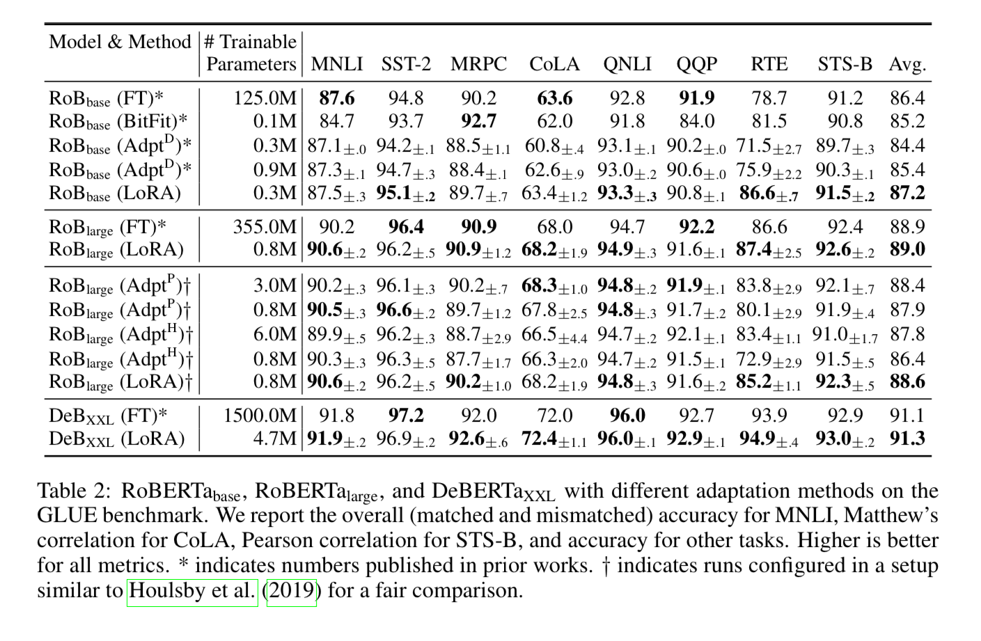
We won’t get into all the adapters they compared against, but you can see LoRA is competitive if not better than many of them when used on RoBERTa
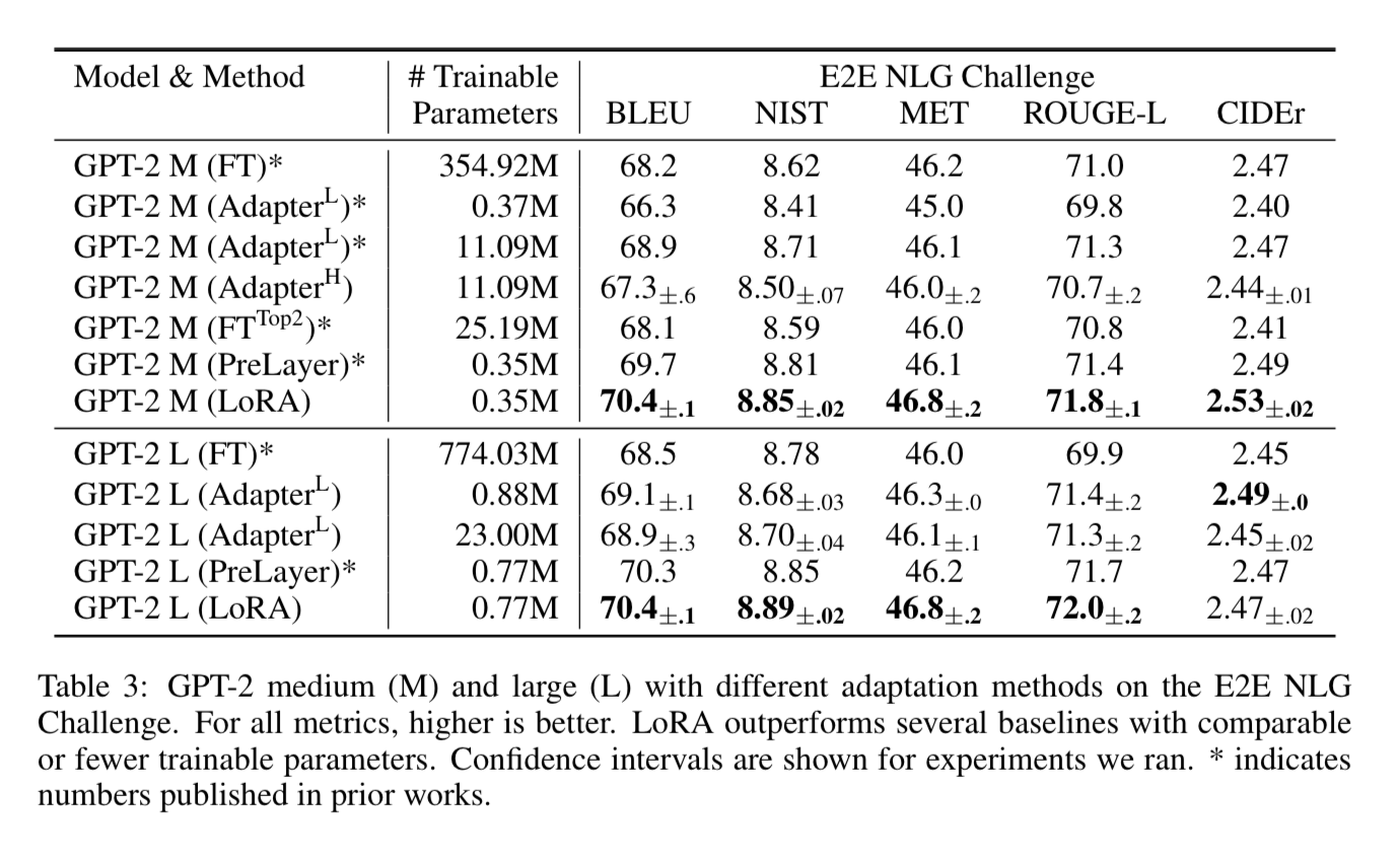
Even though the number of trainable parameters is much smaller, you can see the performance when applied GPT-2 exceeds a lot of the Adapter and PreLayer approaches.
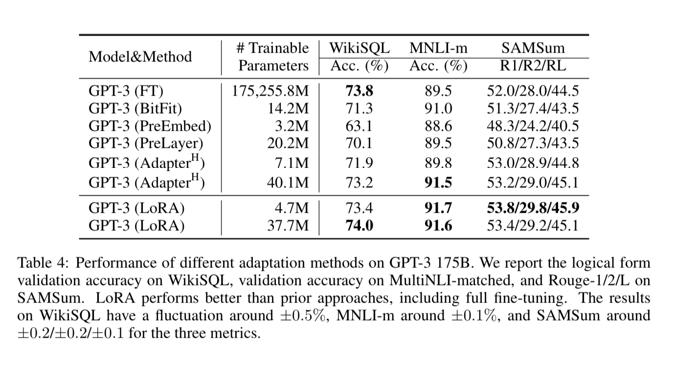
Same goes for GPT-3 on the tasks mentioned above. GPT-3 is much more expensive to run, so this is why they are not consistent in which benchmarks they apply it to.
What about prompt engineering?
They acknowledge that prompt engineering can be used to maximize a general models performance on a specific task, and state that fine-tuning GPT-3 is not very feasible to compare to prompt engineering, so there had not been a lot of comparisons done between prompting and fine-tuning.
David on the call mentioned that prompt engineering is less robust and more susceptible to prompt injection hacks than full fine tuning.
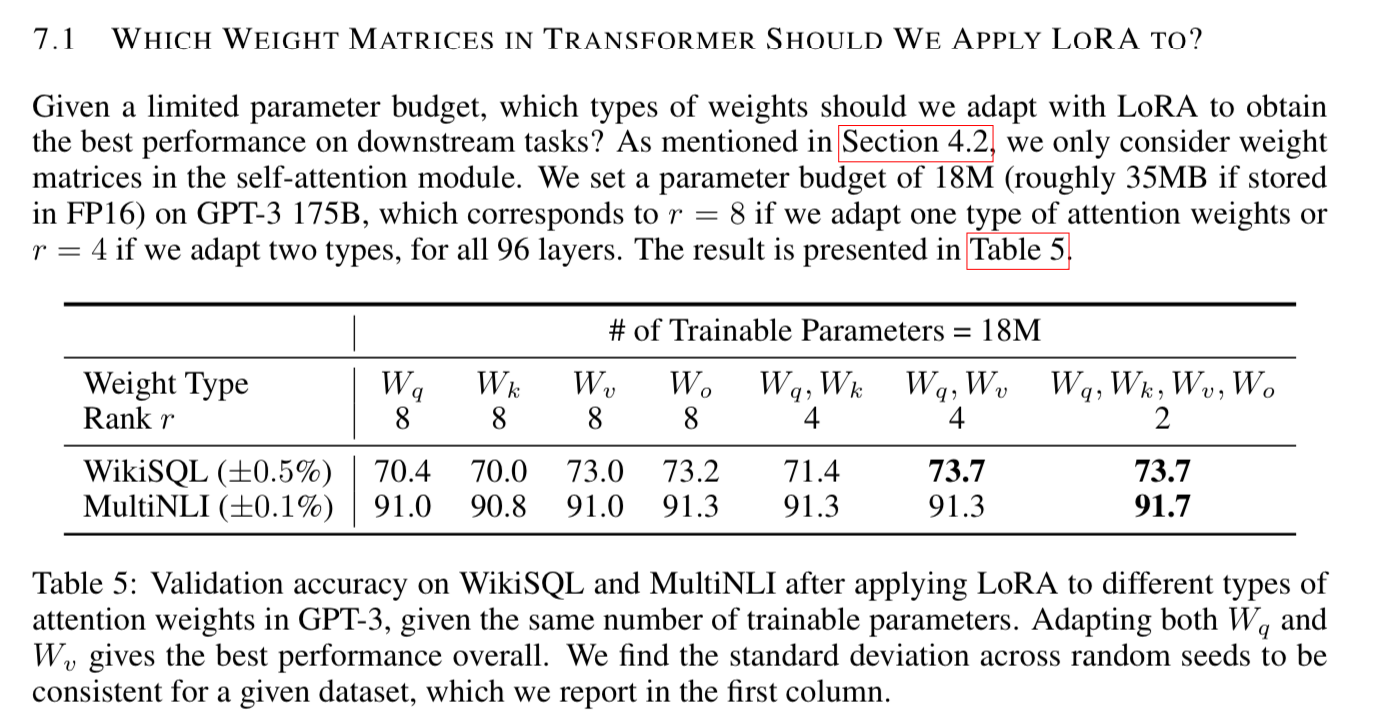
What rank to use and which weights to apply them to?
It’s kind of surprising the lower rank outperforms higher rank when they were evaluating.
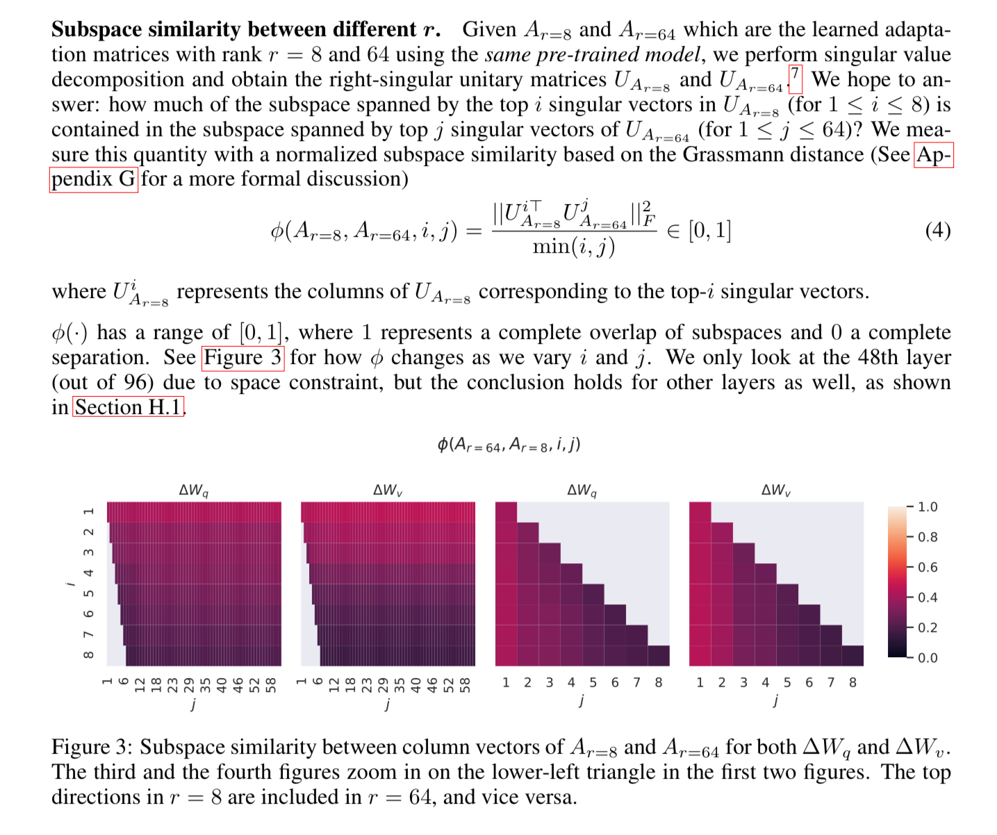
Subspace Similarity
They used singular value decomposition to try to answer how much of the subspace is spanned by the top i singular vectors, and found that if you look at the similarity of the vectors, they are quite high, until you get to that dimension of 1, which is maybe why lower rank performs better.
Here’s another visualization of the subspace similarity between column vectors. You can see, a lot of them have value close to zero, meaning they are very similar, and only those top ranks show differences.
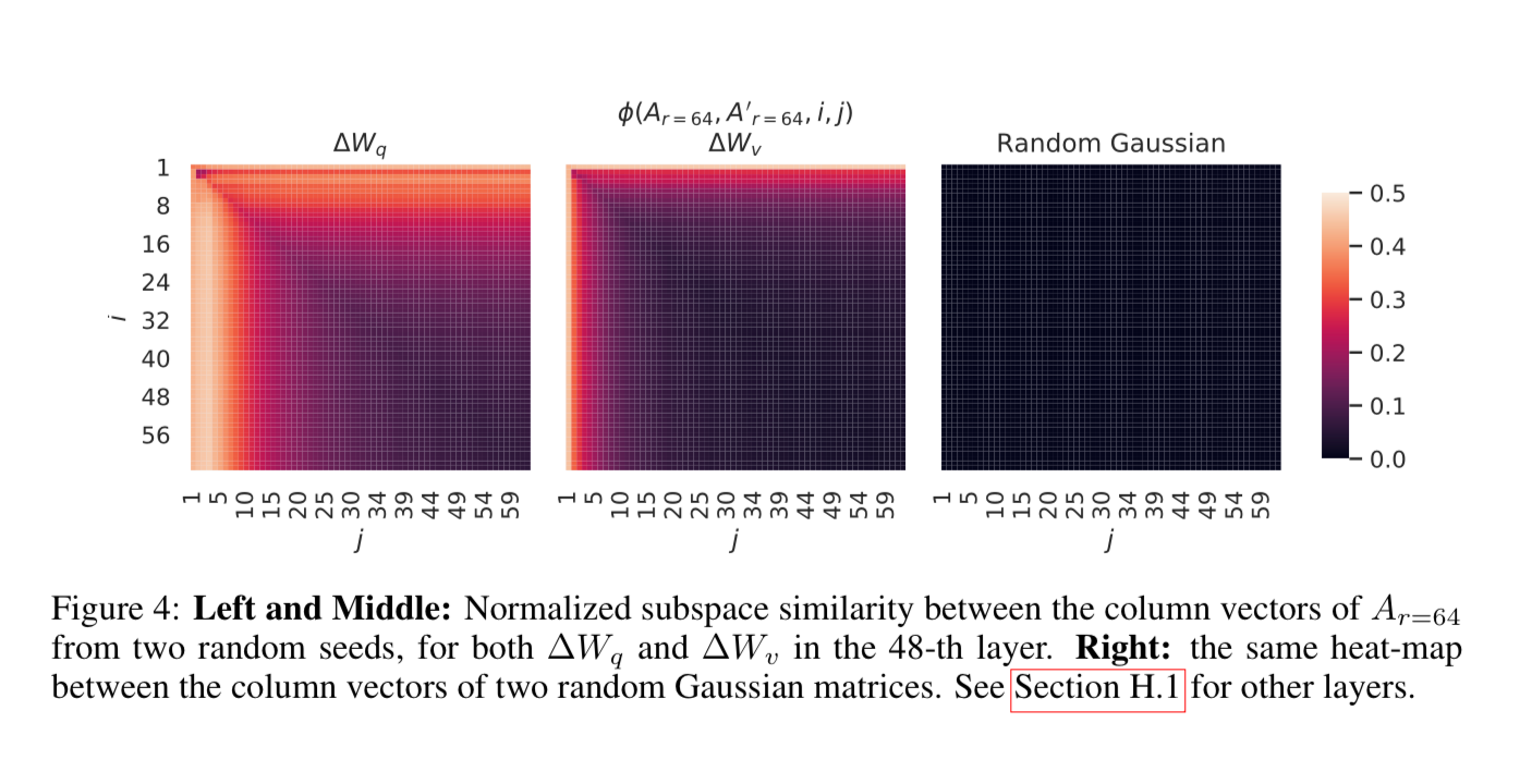
These studies on the weights beg the question of how many parameters are really needed for a large language model in general, if so many of them are linearly dependent.
Conclusion and Future Work
Fine-tuning large language models is prohibitively expensive, especially if you want to switch between different tasks.
LoRA helps reduce the training cost, and quick task switching.
Since LoRA is a technique independent of architecture, it can be used in combination with many other approaches and models.
The mechanism behind fine-tuning or LoRA is far from clear, but they believe that their studies of the rank of matrices make it more tractable to answer these questions than full fine tuning.
They feel there are many other parts of the model you could apply LoRA to, and they picked a lot of their settings with heuristics.
It has helped me experiment with fine-tuning Llama without blowing up the hardware requirements, and we have seen many people adapt it to stable diffusion for image generation, and I feel like many cloud services might be using it under the hood to improve accuracy for different tasks.
Who is Oxen.ai?
Oxen.ai is an open source project aimed at solving some of the challenges with iterating on and curating machine learning datasets. At its core Oxen is a lightning fast data version control tool optimized for large unstructured datasets. We are currently working on collaboration workflows to enable the high quality, curated public and private data repositories to advance the field of AI, while keeping all the data accessible and auditable.
If you would like to learn more, star us on GitHub or head to Oxen.ai and create an account.